Lab: Analysis of variance

With solutions

The goal of this lab is to learn how to implement analysis of variance (ANOVA) in R.

Conceptually, ANOVA is essentially an extension of the two-sample \(t\) test to arbitrarily many means; however, the model is a bit more complex and with more moving parts.

We’ll use the chicks dataset to illustrate and you’ll reproduce using the anorexia dataset.

library(tidyverse)
library(effectsize)
load('data/chicks-20d.RData')
load('data/anorexia.RData')

Preliminaries

Analysis of variance should start with a brief descriptive analysis: visualization of the data by group and calculation of summary statistics.

Side-by-side boxplots can be constructed in exactly the same way we saw before:

# side-by-side boxplots
boxplot(weight ~ diet, data = chicks)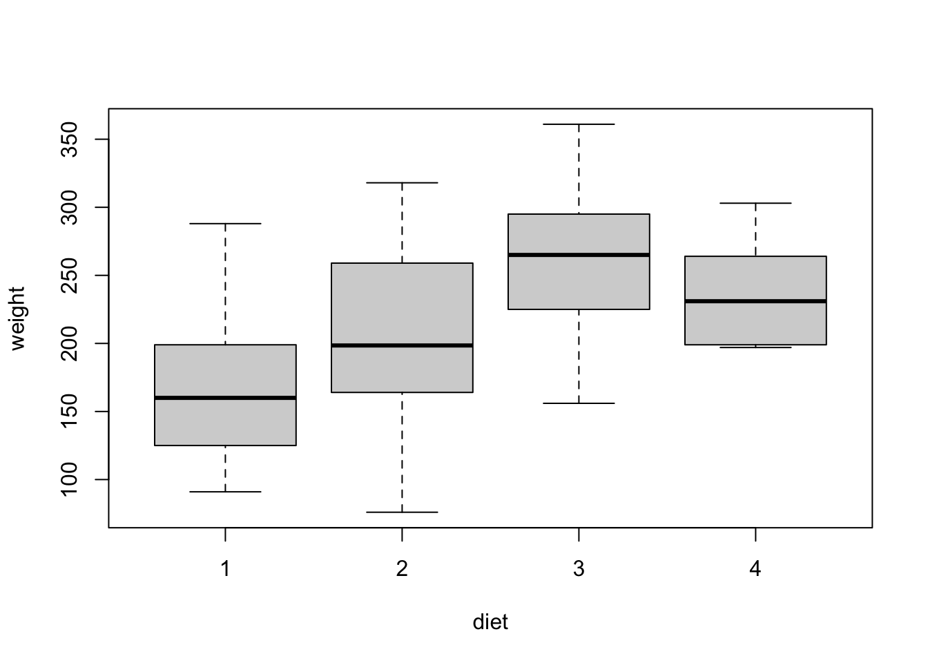

While it is possible to use split(...) like we did for the \(t\) test, there is a more efficient way to compute grouped summary statistics: group_by and summarize from the tidyverse package:

# groupwise summaries: mean, sd, and n
chicks |>
  group_by(diet) |>
  summarize(mean = mean(weight),
            sd = sd(weight),
            n = length(weight))

# A tibble: 4 × 4
  diet   mean    sd     n
  <fct> <dbl> <dbl> <int>
1 1      170.  55.4    17
2 2      206.  70.3    10
3 3      259.  65.2    10
4 4      234.  37.6     9

The basic syntax here is:

group_by(...) takes as its argument the grouping variable exactly as it is named in the dataset
summarize(...) takes a list of arguments of the form NAME = function(VARIABLE)

The above shows calculation of group means, standard deviations, and sample sizes by diet; however, you can add other summary statistics if you wish.

In this case, group sizes are modest but the distributions look similar across groups, so ANOVA model assumptions seem reasonable.

Your turn

Produce descriptive summaries – boxplots and summary statistics – for the change variable in the anorexia dataset. (This is the difference between pre-treatment and post-treatment weight, computed as post - pre.) Assess whether model assumptions for ANOVA are reasonable.

Solution

# boxplots by group
boxplot(change ~ treat, data = anorexia)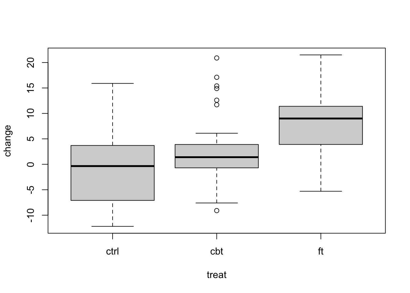

# groupwise summaries: mean, sd, and n
anorexia |>
  group_by(treat) |>
  summarize(mean = mean(change),
            sd = sd(change),
            n = length(change))

# A tibble: 3 × 4
  treat   mean    sd     n
  <fct>  <dbl> <dbl> <int>
1 ctrl  -0.450  7.99    26
2 cbt    3.01   7.31    29
3 ft     7.26   7.16    17

The distribution for the CBT group looks a little different than the others – more concentrated but with outliers – yet summary statistics indicate similar spread. Sample sizes are moderate (actually somewhat large for ANOVA).

Analysis of Variance

Fitting ANOVA models with `aov(...)`

Fitting an ANOVA model is fairly straightforward in R. The command is:

aov(formula = <RESPONSE> ~ <GROUP>, data = <DATAFRAME>)

Where <RESPONSE> is the name of the variable of interest in <DATAFRAME> and <GROUP> is the name of the grouping variable. These should match exactly the syntax you use to make your boxplot.

# fit anova model
fit.chicks <- aov(formula = weight ~ diet, data = chicks)
fit.chicks

Call:
   aov(formula = weight ~ diet, data = chicks)

Terms:
                     diet Residuals
Sum of Squares   55881.02 143190.31
Deg. of Freedom         3        42

Residual standard error: 58.38915
Estimated effects may be unbalanced

The fitted ANOVA model displays only sums of squares, degrees of freedom, and \(\sqrt{MSE}\), which is a pooled estimate of the standard deviation of data values about the group means (“residual standard error”).

Omnibus \(F\) test

For the omnibus test of no effect, we need the ANVOA table:

# construct anova table
summary.aov(fit.chicks)

            Df Sum Sq Mean Sq F value  Pr(>F)   
diet         3  55881   18627   5.464 0.00291 **
Residuals   42 143190    3409                   
---
Signif. codes:  0 '***' 0.001 '**' 0.01 '*' 0.05 '.' 0.1 ' ' 1

At the 1% level, the test is significant (\(H_0\) rejected) since \(p < 0.01\), so the result is:

The data provide evidence that diet has an effect on mean weight among chicks (F = 5.46 on 3 and 42 degrees of freedom, p = 0.00291).

Your turn

Test for an effect of therapeutic treatment on mean weight change among anorexia patients at the 5% level. Fit the ANOVA model using aov(...) and generate the ANOVA table using summary.aov(...). Interpret the result in context.

Solution

# fit anova model
fit.anorexia <- aov(change ~ treat, data = anorexia)

# construct anova table
summary(fit.anorexia)

            Df Sum Sq Mean Sq F value Pr(>F)   
treat        2    615  307.32   5.422 0.0065 **
Residuals   69   3911   56.68                  
---
Signif. codes:  0 '***' 0.001 '**' 0.01 '*' 0.05 '.' 0.1 ' ' 1

The data provide evidence of an effect of therapy in treating anorexia (F = 5.422 on 2 and 69 df, p = 0.0065).

Estimating effect size

Once you’ve inferred an effect (and sometimes even if you haven’t), a natural question is, “how much of an effect is there?”

The most common effect size measure is \(\eta^2\) (“eta-squared”), or the proportion of total variability attributable to groups: \[ \eta^2 = \frac{SSG}{SST} \] Since in a one-way ANOVA, \(SST = SSG + SSE\), we could get an estimate directly from the table:

# anova table
summary(fit.chicks)

            Df Sum Sq Mean Sq F value  Pr(>F)   
diet         3  55881   18627   5.464 0.00291 **
Residuals   42 143190    3409                   
---
Signif. codes:  0 '***' 0.001 '**' 0.01 '*' 0.05 '.' 0.1 ' ' 1

\[ \eta^2 = \frac{55881}{55881 + 143190} = 0.2807089 \] But there is a handy function that performs this calculation for us using the fitted model:

# estimate effect size
eta_squared(fit.chicks, partial = F)

# Effect Size for ANOVA (Type I)

Parameter | Eta2 |       95% CI
-------------------------------
diet      | 0.28 | [0.08, 1.00]

- One-sided CIs: upper bound fixed at [1.00].

The confidence interval is for the population \(\eta^2\) and is interpreted as follows:

With 95% confidence, diet accounts for an estimated 8% or more of total variation in chick weights at 20 days.

By default, a one-sided interval is reported; this can be changed if desired by adding an alternative = ... argument. Similarly

# adjust confidence interval for effect size
eta_squared(fit.chicks, partial = F, alternative = 'two.sided', ci = 0.9)

# Effect Size for ANOVA (Type I)

Parameter | Eta2 |       90% CI
-------------------------------
diet      | 0.28 | [0.08, 0.43]

Thus:

With 90% confidence, diet accounts for an estimated 8% to 43% of total variation in chick weights at 20 days.

Your turn

Estimate the effect size of therapy on weight change among anorexia patients. Provide a two-sided 95% confidence interval and interpret the interval in context.

Solution

# estimate effect size
eta_squared(fit.anorexia, partial = F, ci = 0.95, alternative = 'two.sided')

# Effect Size for ANOVA (Type I)

Parameter | Eta2 |       95% CI
-------------------------------
treat     | 0.14 | [0.01, 0.28]

With 95% confidence, therapeutic treatment accounts for an estimated 1% to 28% of total variation in weight change.

Study design power analysis

To power a study for a specified effect size \(\eta_0^2\), use the simple heuristic:

\[ \begin{align*} MSG &= \eta_0^2 \\ MSE &= 1 - \eta_0^2\ \end{align*} \]

This works well provided the sample size \(n\) is large relative to the number of groups \(k\), which is almost always the case.

For example, to redesign the chick weight study to detect an effect size of \(\eta^2 = 0.15\) (diets account for 15% of total variation) 90% of the time, we’d need 28 chicks in each group or 112 in total.

# power calculation
power.anova.test(groups = 4,
                 sig.level = 0.05,
                 power = 0.9,
                 between.var = 0.15,
                 within.var = 0.85)


     Balanced one-way analysis of variance power calculation 

         groups = 4
              n = 27.76682
    between.var = 0.15
     within.var = 0.85
      sig.level = 0.05
          power = 0.9

NOTE: n is number in each group

Your turn

Suppose you’re designing a follow-up to the anorexia study in which you add two more therapies to the experiment. Suppose also that a clinically significant effect size is 5% of total variation in weight loss. Determine the number of patients you’d need to enroll to detect this effect 80% of the time using a 5% level test.

Solution

# power calculation
power.anova.test(groups = 5,
                 sig.level = 0.05,
                 power = 0.8,
                 between.var = 0.05,
                 within.var = 0.95)


     Balanced one-way analysis of variance power calculation 

         groups = 5
              n = 57.64931
    between.var = 0.05
     within.var = 0.95
      sig.level = 0.05
          power = 0.8

NOTE: n is number in each group

Answer: 58 patients per group or 290 in total.

Preliminaries

Analysis of Variance

Fitting ANOVA models with aov(...)

Omnibus \(F\) test

Estimating effect size

Study design power analysis

Fitting ANOVA models with `aov(...)`