load('data/finch.RData')
load('data/temps2.RData')Lab: Two-sample inference
With solutions
This lab focuses on two-sample inference for differences in population means. We’ll use two datasets for which we will consider two-sample comparisons:
finch: mean finch beak depths in generations before and after a drought on Daphne Majortemps: body temperatures and heart rates for men and women
Examples will utilize the finch data; you’ll practice using the temps data.
Checking assumptions
A two-sample \(t\)-test can be used whenever two one-sample tests are appropriate. So, to check assumptions, we need to inspect the frequency distributions of the variable of interest in both samples.
To do that, we’ll need to separate the samples. This can be done by partitioning observations of beak depth by year.
# split observations by year
f.year <- finch$year
f.depth <- finch$depth
f.split <- split(f.depth, f.year)

# retrieve depth measurements from each year
depth.1978 <- f.split$`1978`
depth.1976 <- f.split$`1976`
We could then check assumptions by comparing histograms:
# make histograms
hist(depth.1978)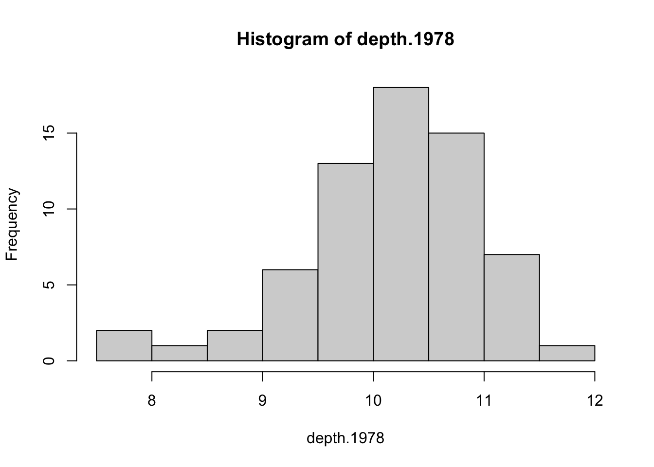
hist(depth.1976)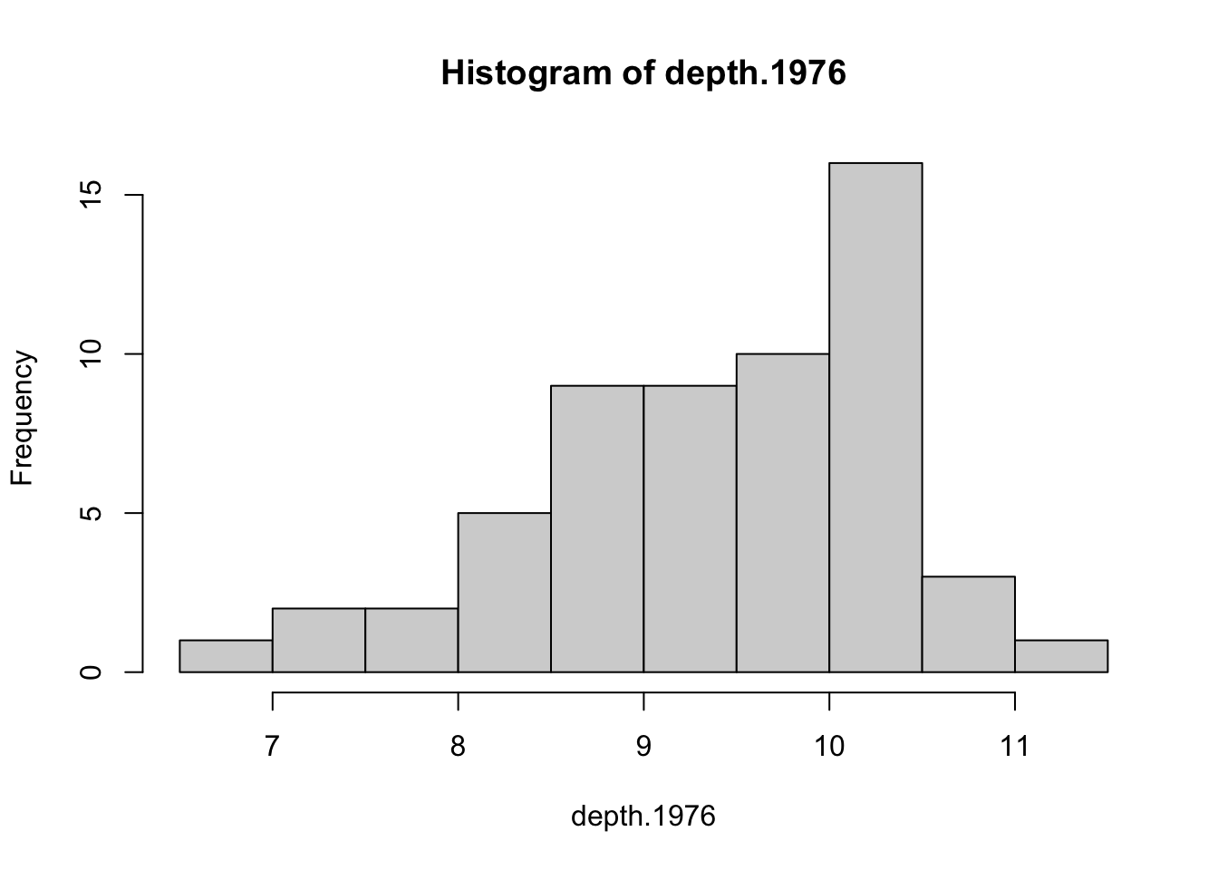
While there is a bit of left skewness, the sample sizes are large enough that it’s not a concern.
Your turn
Partition the temps data by sex and make histograms of the heart rates. Comment on whether assumptions seem to be met.
Solution
# split observations of heart rate by sex
hr <- temps$heart.rate
sex <- temps$sex
hr.split <- split(hr, sex)

# retrieve heart rate measurements from each group
hr.m <- hr.split$male
hr.f <- hr.split$female

# make histograms and compare
hist(hr.f)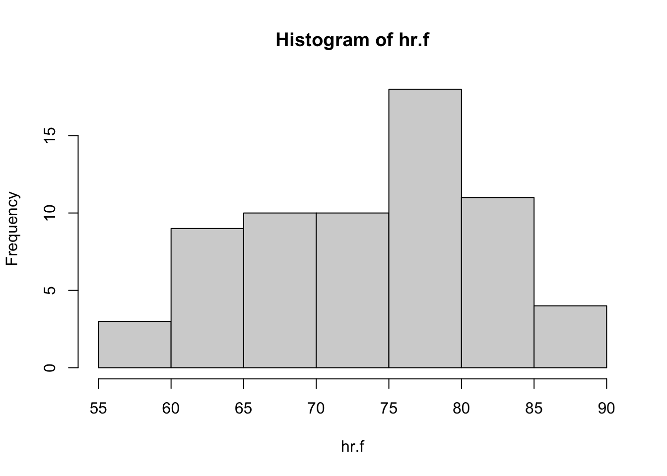
hist(hr.m)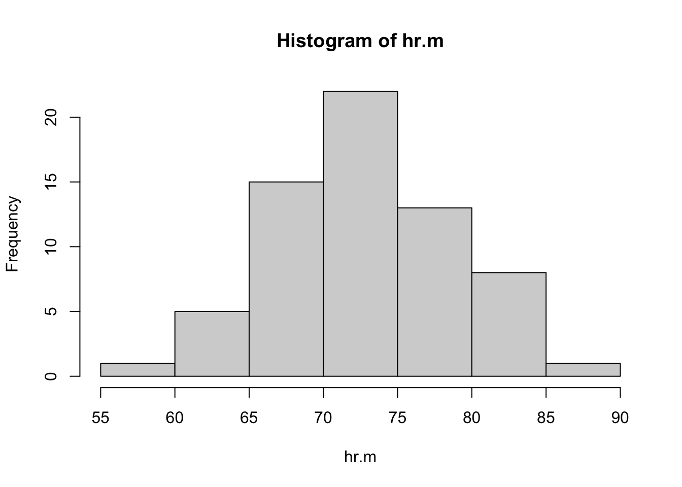
Sample sizes are large and both distributions are unimodal, so the \(t\) test is reasonable here. There is a bit of left skewness for the distribution of heart rates among women; by contrast, the distribution for men looks symmetric. Neither distribution includes outliers.
Exploratory plots
When comparing histograms, it’s difficult to judge if there appears to be a difference between samples/groups. The eye has to jump back and forth, and the centers are not always visually obvious.
Side-by-side boxplots provide a nice alternative that makes it easy to compare the groups for location differences (and thus different means). This can be done with the original dataset (no need to partition):
# side-by-side boxplots
boxplot(depth ~ year, data = finch, horizontal = T)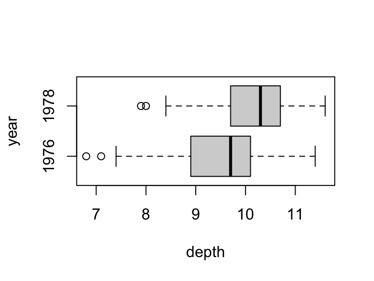
It looks like there is a clear difference – beak depths are greater in 1978 – so now the question is simply whether that difference is statistically significant relative to the sampling variation in our estimates.
As an aside, the syntax y ~ x is called a formula in R. You can read it verbally as “y depends on x”; in the above example, we would read depth ~ year as saying “depth depends on year”.
Your turn
Make side-by-side boxplots for heart rate and reassess test assumptions.
Solution
# side-by-side boxplots
boxplot(heart.rate ~ sex, data = temps, horizontal = T)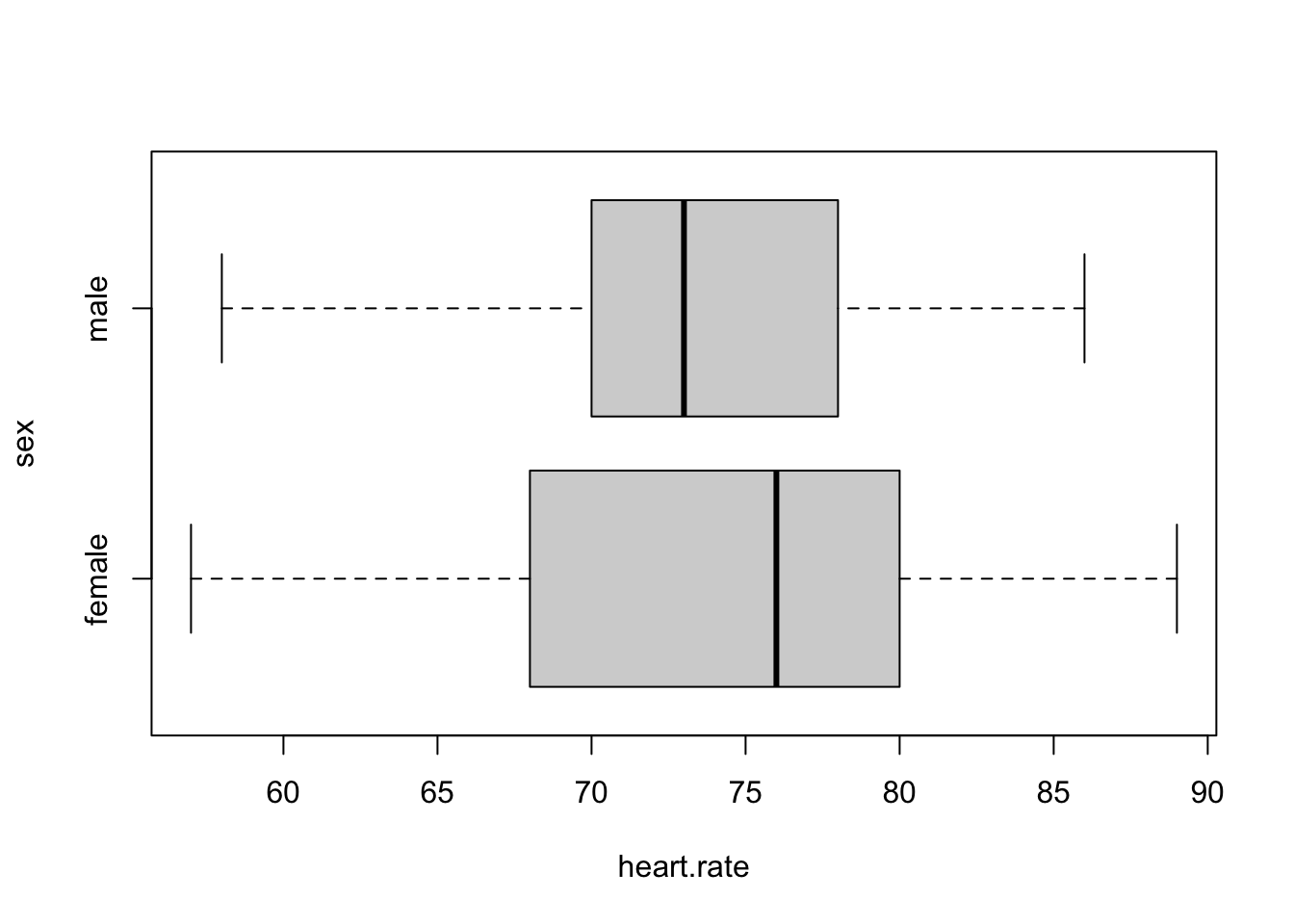
Test assumptions still seem reasonable; it’s not clear that there’s much of a difference by sex, so it would be a little surprising if a statistical test rejected the hypothesis of no difference.
Two-sample \(t\)-tests
To test whether the drought imposed selection pressure on the finch population, we want to know whether finch beak depth increased after the drought, i.e.,
\[ \begin{cases} H_0: &\mu_{1976} = \mu_{1978} \\ H_A: &\mu_{1976} < \mu_{1978} \end{cases} \]
We can perform the test using t.test(...) with a formula in which the variable of interest is on the left and the grouping variable is on the right.
# perform t test
t.test(formula = depth ~ year,
       data = finch,
       mu = 0,
       alternative = 'less',
       conf.level = 0.95)
    Welch Two Sample t-test

data:  depth by year
t = -4.5727, df = 111.79, p-value = 6.255e-06
alternative hypothesis: true difference in means between group 1976 and group 1978 is less than 0
95 percent confidence interval:
       -Inf -0.4698812
sample estimates:
mean in group 1976 mean in group 1978
          9.453448          10.190769
Notice two subtleties:
- we need to supply a
dataargument; the formula won’t work if R doesn’t know where to find the variables of interest - the alternative is specified as
less; this is because the first group in the data is 1976, so the alternative reads “mean in 1976 is less than mean in 1978”; to determine which group comes first, look at which point estimate is printed first in the output
The point estimates and standard error can be retrieved by storing the output of t.test(...).
# store t test result
tt.rslt <- t.test(formula = depth ~ year,
                  data = finch,
                  mu = 0,
                  alternative = 'less',
                  conf.level = 0.95)

# print results
tt.rslt
    Welch Two Sample t-test

data:  depth by year
t = -4.5727, df = 111.79, p-value = 6.255e-06
alternative hypothesis: true difference in means between group 1976 and group 1978 is less than 0
95 percent confidence interval:
       -Inf -0.4698812
sample estimates:
mean in group 1976 mean in group 1978
          9.453448          10.190769
# estimates
tt.rslt$estimatemean in group 1976 mean in group 1978
9.453448 10.190769 # estimate for difference in means
tt.rslt$estimate |> diff()mean in group 1978
0.737321 # standard error for estimate of difference in means
tt.rslt$stderr[1] 0.1612445We’d report the test result as follows:
The data provide evidence that mean beak depth increased in the generation of finches following the drought (T = -4.5727 on 111.79 degrees of freedom, p < 0.0001). With 95% confidence, the mean beak depth is estimated to have increased by at least 0.4699 mm, with a point estiamte of 0.7373 mm (SE 0.1612).
Your turn
Test whether mean heart rate differs between men and women at the 1% significance level. (Make sure your interval estimate is consistent with the level and alternative of your test.) Report the test result, confidence interval, and point estimate and standard error for the difference in means.
Solution
# store t test result
tt.rslt <- t.test(formula = heart.rate ~ sex,
                  data = temps,
                  mu = 0,
                  alternative = 'two.sided',
                  conf.level = 0.99)

# print results
tt.rslt
    Welch Two Sample t-test

data:  heart.rate by sex
t = 0.63191, df = 116.7, p-value = 0.5287
alternative hypothesis: true difference in means between group female and group male is not equal to 0
99 percent confidence interval:
 -2.466825  4.036055
sample estimates:
mean in group female   mean in group male
            74.15385             73.36923
# estimates
tt.rslt$estimatemean in group female mean in group male
74.15385 73.36923 # estimate for difference in means
tt.rslt$estimate |> diff()mean in group male
-0.7846154 # standard error for estimate of difference in means
tt.rslt$stderr[1] 1.241665Test interpretation:
The data provide no evidence that heart rate differs by sex (T = 0.63 on 116.7 degrees of freedom, p = 0.5287).
Interval interpretation:
With 95% confidence, the difference in mean heart rate between women and men is estimated to be between -2.47 and 4.04 bpm.
Point estimate:
Mean heart rate is estimated to be 0.78 bpm higher among women compared with men (SE 1.24).
Study design power analysis
In the analysis above, the estimated difference in mean beak depth is about 0.5mm. How many birds should we have measured to detect a difference of this magnitude at least 90% of the time?
The power.t.test(...) function will do the calculation given the requisite inputs:
delta: target difference in means \(\delta\)sd: an estimate of the population standard deviationsig.level: significance level of the testtype: type of t-test, should be'two.sample'alternative: either'one.sided'or'two.sided'power: target power
In the prior analysis, we used a one-sided test; the level was never mentioned explicitly because the p-value was so small. Let’s imagine it was 5%.
For a conservative power calculation, we’ll use the larger of the two sample standard deviations from the previous study.
# choose larger of the two sds
sd(depth.1976)
[1] 0.9624923sd(depth.1978)[1] 0.8073342Now we have all the inputs:
delta: target difference is 0.5mmsd: larger of the two groups was 0.96sig.level: we’ll consider the usual 5%type: two sample testalternative: one sidedpower: 90%
Providing them to power.t.test:
# power calculation
power.t.test(delta = 0.5,
             sd = 0.96,
             sig.level = 0.05,
             type = 'two.sample',
             alternative = 'one.sided',
             power = 0.9)
     Two-sample t test power calculation

              n = 63.82749
          delta = 0.5
             sd = 0.96
      sig.level = 0.05
          power = 0.9
    alternative = one.sided

NOTE: n is number in *each* group
Rounding n to the nearest whole number, we’d need 64 individuals in each year to achieve the specified power.
Your turn
Suppose the smallest clinically relevant difference in mean heart rate is 5bpm. How many individuals should we sample in each group to detect a clinically relevant difference using the test performed above 90% of the time?
Solution
# find larger sd of two groups
sd(hr.f)
[1] 8.105227sd(hr.m)[1] 5.875184# specify test attributes
power.t.test(delta = 5,
sd = 8,
sig.level = 0.01,
type = 'two.sample',
alternative = 'two.sided',
power = 0.9)
     Two-sample t test power calculation

              n = 77.85929
          delta = 5
             sd = 8
      sig.level = 0.01
          power = 0.9
    alternative = two.sided

NOTE: n is number in *each* group
The difference of interest is \(\delta = 5\), and the larger standard deviation is around 8bpm. Above, we used a two-sided test with a 1% significance level. Providing these inputs with power \(\beta = 0.9\) yields that at least 78 individuals in each group are needed to detect a clinically relevant difference at least 90% of the time.