Lab 5: Two-sample inference

With solutions

Author

Your Name Here

Before you begin

Fill in the author and calpoly-id fields at the very top of this file. Replace "Your Name Here" with your full name and "yourpolynetid" with your Cal Poly username (the part of your email before @calpoly.edu, e.g. jdoe01). Your submission cannot be matched to your record without this.

Where a “Your turn” asks you to save a result by a specific name (shown in bold), use the exact name given — your work is checked automatically.

This lab focuses on two-sample inference for differences in population means. We’ll use two datasets:

finch: beak depths of Darwin’s finches on Daphne Major, measured before and after a drought
temps: body temperatures and heart rates for men and women

load('data/finch.RData')
load('data/temps2.RData')

Examples use the finch data; you’ll practice using temps.

Exploratory plots

How do beak depths compare between years?

Side-by-side boxplots give a quick visual comparison of two or more groups. The formula syntax y ~ x specifies the response and grouping variables:

# side-by-side boxplots
boxplot(depth ~ year, data = finch, horizontal = TRUE)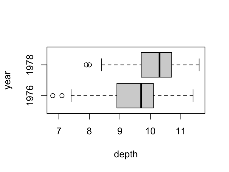

Boxplots also serve as a quick assumption check — look for outliers or extreme skewness within groups, which would make the \(t\) test less reliable.

It looks like there is a clear difference — beak depths are greater in 1978. The question is whether that difference is statistically significant relative to sampling variation.

How do heart rates compare between men and women?

Your turn 1

Make side-by-side boxplots of heart.rate by sex from the temps data. Is there a visible difference between groups? Do the distributions look compatible with using a \(t\) test?

Solution

# side-by-side boxplots
boxplot(heart.rate ~ sex, data = temps, horizontal = TRUE)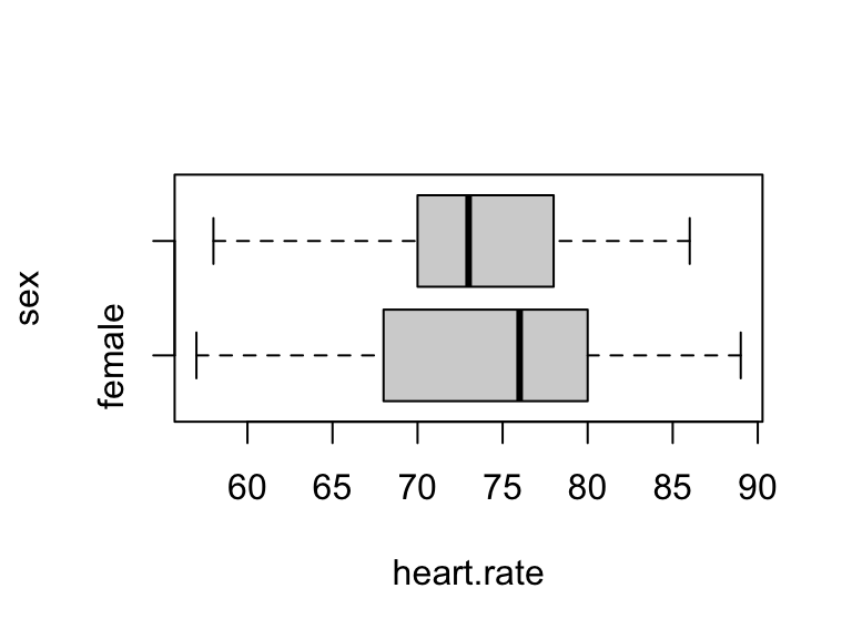

The distributions are unimodal with no extreme outliers or skewness, and the sample sizes are large, so the \(t\) test is appropriate. It’s not clear that there’s much of a difference by sex.

Two-sample \(t\)-tests

Did the drought change mean finch beak depth?

To test whether the drought imposed selection pressure on the finch population, we want to know whether beak depth increased after the drought:

\[ \begin{cases} H_0: &\mu_{1976} = \mu_{1978} \\ H_A: &\mu_{1976} < \mu_{1978} \end{cases} \]

t.test(...) accepts a formula interface identical to boxplot(...). The alternative is specified relative to the first group in the data — check which point estimate is printed first in the output to confirm the ordering.

# store and print t test result
tt.finch <- t.test(depth ~ year, data = finch, alternative = 'less')
tt.finch


    Welch Two Sample t-test

data:  depth by year
t = -4.5727, df = 111.79, p-value = 6.255e-06
alternative hypothesis: true difference in means between group 1976 and group 1978 is less than 0
95 percent confidence interval:
       -Inf -0.4698812
sample estimates:
mean in group 1976 mean in group 1978 
          9.453448          10.190769

The p-value is far below 0.05:

The data provide evidence that mean beak depth increased in the generation of finches following the drought (T = −4.573 on 111.79 df, p < 0.0001).

Does mean heart rate differ between men and women?

Your turn 2 [L5]

Test whether mean heart rate differs between men and women at the 1% significance level. Store the full test result as tt.hr. Interpret the result in one sentence.

Solution

# two-sided two-sample t-test at the 1% level
tt.hr <- t.test(heart.rate ~ sex, data = temps, conf.level = 0.99)
tt.hr


    Welch Two Sample t-test

data:  heart.rate by sex
t = 0.63191, df = 116.7, p-value = 0.5287
alternative hypothesis: true difference in means between group female and group male is not equal to 0
99 percent confidence interval:
 -2.466825  4.036055
sample estimates:
mean in group female   mean in group male 
            74.15385             73.36923

The data do not provide evidence that mean heart rate differs by sex (T = 0.629 on 116.7 df, p = 0.531).

Estimates and confidence intervals

What is the estimated difference, and how precise is it?

The output of t.test(...) includes a confidence interval along with the test. Once the result is stored, we can also extract the point estimates and standard error for the difference in means:

# group means
tt.finch$estimate

mean in group 1976 mean in group 1978 
          9.453448          10.190769

# estimated difference (1978 − 1976)
tt.finch$estimate |> diff()

mean in group 1978 
          0.737321

# standard error of the estimated difference
tt.finch$stderr

[1] 0.1612445

We report the estimate in context:

With 95% confidence, mean beak depth is estimated to have increased by at least 0.470 mm following the drought, with a point estimate of 0.737 mm (SE 0.161).

What is the estimated difference in heart rates, and how precise is it?

Your turn 3

From your stored result tt.hr, extract:

the group means
the estimated difference in means (women − men)
the standard error of the estimated difference

Write one sentence reporting the point estimate and SE in context.

Solution

# group means
tt.hr$estimate

mean in group female   mean in group male 
            74.15385             73.36923

# estimated difference (women − men)
tt.hr$estimate |> diff()

mean in group male 
        -0.7846154

# standard error
tt.hr$stderr

[1] 1.241665

Mean heart rate is estimated to be 0.78 bpm higher among women compared with men (SE 1.24 bpm).

Submitting this assignment

Save the file (Ctrl+S / Cmd+S).
Render to PDF: click Render or press Ctrl+Shift+K / Cmd+Shift+K.
Download both files: in the Files panel, check the .qmd and PDF, then click More ▾ → Export….
Upload the PDF to the Gradescope assignment for this lab.
Upload the .qmd file to the course submission link.