load('data/temps.RData')
head(temps)
body.temp sex heart.rate
1 98.8 female 69
2 98.6 female 85
3 98.4 male 68
4 97.2 female 66
5 99.5 male 75
6 97.1 male 82With solutions
The focus of this lab is the one-sample \(t\) test for a population mean. We’ll use the temps dataset to illustrate.
load('data/temps.RData')
head(temps) body.temp sex heart.rate
1 98.8 female 69
2 98.6 female 85
3 98.4 male 68
4 97.2 female 66
5 99.5 male 75
6 97.1 male 82The \(t\) test only makes sense for unimodal population distributions of numeric variables. Beyond that, the test is based on the assumption that either the underlying population distribution is symmetric or the sample size is not too small, so we need to check two things:
“Too small” is relative to just how much funny business you see in the distribution of values: more pronounced skewness or outliers means that more data are required for the test to work well.
For sample sizes, here is a rule of thumb for the \(t\)-test:
For shape, here are a few rules of thumb:
in the “small” regime, the distribution should be symmetric and not include outliers
in the ‘modest’ regime, the distribution should not include extreme outliers
in the ‘large’ regime, there are no restrictions on the
For the body temperature data, we have 39 observations, which is neither small nor large but modest. So, we don’t need to be too sensitive unless extreme outliers are present.
# extract temperature variable
btemp <- temps$body.temp

# location measures
summary(btemp)
Min. 1st Qu. Median Mean 3rd Qu. Max.
96.40 97.85 98.40 98.41 99.00 100.80 # histogram
hist(btemp, breaks = 10)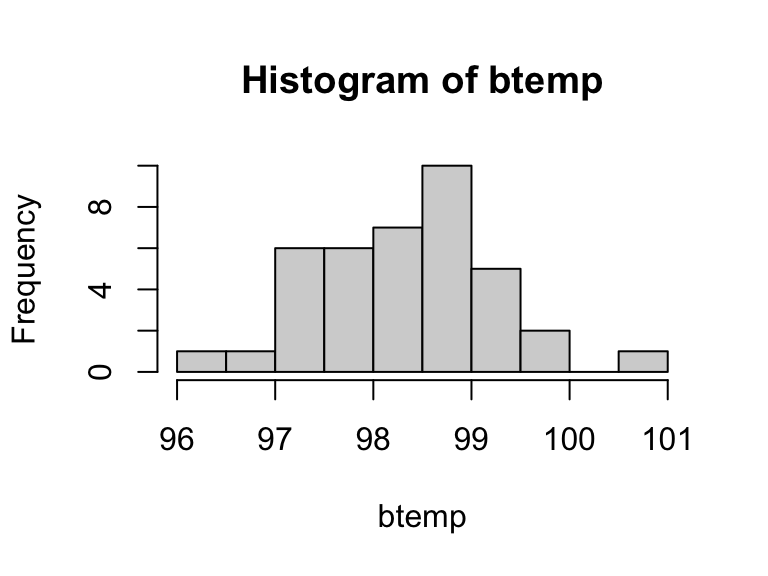
The histogram suggests a unimodal population, so conceptually the test is sensible; moreover, there’s no indication of strong skewness or outliers, so the test should work just fine.
Check the distribution of the heart.rate variable. Assess whether the \(t\) test is appropriate, taking account of the sample size.
# extract heartrate variable
hrate <- temps$heart.rate

# location measures
summary(hrate)
Min. 1st Qu. Median Mean 3rd Qu. Max.
57.00 69.50 75.00 73.95 79.00 86.00 # histogram
hist(hrate, breaks = 6)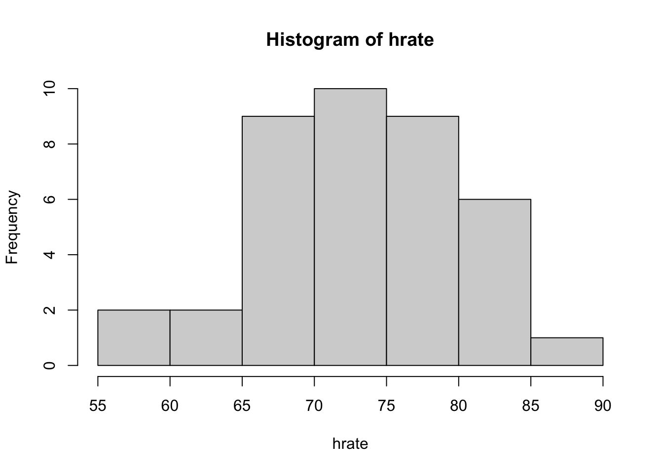
Since there is a modest amount of data, the shape of the distribution and presence of outliers matter. However, the histogram of heart rates is fairly symmetric and there are no outliers, so the \(t\) test is appropriate.
For the one-sample \(t\)-test we use the test statistic:
\[ T = \frac{\bar{x} - \mu_0}{SE(\bar{x})} \]
In this expression \(\mu_0\) is a placeholder for the hypothesized value of \(\mu\) in any particular problem. To test whether the mean body temperature is 98.6°F, substitute \(\mu_0 = 98.6\):
# store sample mean and standard error
btemp.mean <- mean(btemp)
btemp.mean.se <- sd(btemp)/sqrt(length(btemp))

# calculate t statistic
btemp.tstat <- (btemp.mean - 98.6)/btemp.mean.se
btemp.tstat
[1] -1.328265Take a moment to match the code to the mathematical formula. Then, notice that the result is the same value we obtained in lecture.
First consider the \(t\)-test for a two-sided alternative. The hypotheses are:
\[ \begin{cases} H_0: \mu = 98.6 \\ H_A: \mu \neq 98.6 \end{cases} \]
The \(p\)-value for this test is the proportion of samples for which \(T\) is greater in magnitude than the observed value -1.328. By symmetry of the \(t\) model, this can be computed as:
\[P(|T| > |T_\text{observed}|) = 2\times P(T > |T_\text{observed}|)\] In R:
# two-sided p-value
2*pt(abs(btemp.tstat), df = length(btemp) - 1, lower.tail = F)
[1] 0.1920133Notice that this matches the value from lecture.
Now recall the decision rule for a level \(\alpha\) test:
In this example, if we are performing a level 0.05 test, we’d fail to reject \(H_0\) since \(p \geq 0.05\). We would then report the test result as follows:
The data do not provide evidence that the mean body temperature differs from 98.6°F (T = -1.328 on 38 degrees of freedom, p = 0.192).
Choose a hypothetical mean heart rate between 65 and 75 beats per minute (bpm) and test your hypothesis relative to the two-sided alternative. Interpret your test in context.
Here is a test of whether mean heart rate is 70 beats per minute.
# store sample mean and standard error
hrate.mean <- mean(hrate)
hrate.se <- sd(hrate)/sqrt(length(hrate))

# calculate t statistic
hrate.tstat <- (hrate.mean - 70)/hrate.se

# calculate two-sided p value
2*pt(abs(hrate.tstat), df = length(hrate) - 1, lower.tail = F)
[1] 0.001141458The data provide evidence that mean heart rate differs from 70 bpm (T = 3.519 on 38 df, p = 0.0011).
Now consider testing whether mean body temperature is less than 98.6°F:
\[ \begin{cases} H_0: \mu = 98.6 \\ H_A: \mu < 98.6 \end{cases} \]
We now want to use a lower-sided \(p\)-value that captures how often we’d observe a test statistic less than the observed value:
\[P(T < T_\text{observed})\]
In R:
# lower-sided p-value
pt(btemp.tstat, df = length(btemp) - 1, lower.tail = T)
[1] 0.09600667There are three differences from the two-sided test:
lower.tail = T to return the cumulative frequency of values to the left of the T statisticTo determine the outcome, we apply the same decision rule as before for a level \(\alpha\) test:
In this case, we fail to reject \(H_A\) at level 0.05, and would report this result as follows:
The data do not provide evidence that mean body temperature is less than 98.6°F (T = -1.328 on 38 degrees of freedom, p = 0.096)
Refer back to your two-sided test of mean heart rate. Test whether mean heart rate is less than your hypothesized value and interpret the test in context.
Continuing my example above, one possible solution is to test whether mean heart rate is less than 70 beats per minute.
# calculate lower-sided p value
pt(hrate.tstat, df = length(hrate) - 1, lower.tail = T)
[1] 0.9994293The data do not provide evidence that mean heart rate is less than 70 bpm (T = 3.519 on 38 df, p = 0.9994).
If instead we wanted to test whether mean body temperature is greater than 98.6°F, i.e., to decide between the hypotheses
\[ \begin{cases} H_0: \mu = 98.6 \\ H_A: \mu > 98.6 \end{cases} \]
then we would use an upper-sided \(p\)-value that captures how often we’d observe a test statistic greater than the observed value:
\[P(T > T_\text{observed})\]
In R:
# lower-sided p-value
pt(btemp.tstat, df = length(btemp) - 1, lower.tail = F)
[1] 0.9039933The only difference from the lower-sided test is that we use lower.tail = F to return the cumulative frequency of values to the right of the T statistic. We apply the same decision rule as before for a level \(\alpha\) test:
In this case, we fail to reject \(H_A\) at level 0.05, and would report this result as follows:
The data do not provide evidence that mean body temperature is greater than 98.6°F (T = -1.328 on 38 degrees of freedom, p = 0.904)
Refer back to your two-sided test of mean heart rate. Test whether mean heart rate is greater than your hypothesized value and interpret the test in context.
Continuing my example above, one possible solution is to test whether mean heart rate is greater than 70 beats per minute.
# calculate upper-sided p value
pt(hrate.tstat, df = length(hrate) - 1, lower.tail = F)
[1] 0.0005707291The data provide evidence that mean heart rate is greater than 70 bpm (T = 3.519 on 38 df, p = 0.0006).
The value in learning to compute \(p\)-values by hand is that you gain a better understanding of the mechanics of the test. However, in practice, you’ll usually rely on software.
In R, the function t.test(...) does the job for you and produces a confidence interval to match the test. You need only provide:
The software will do the rest. This cell shows each of the tests performed above. You can verify that the test statistics, degrees of freedom, and \(p\)-values match.
# two-sided test
t.test(btemp, mu = 98.6, alternative = 'two.sided')
    One Sample t-test

data:  btemp
t = -1.3283, df = 38, p-value = 0.192
alternative hypothesis: true mean is not equal to 98.6
95 percent confidence interval:
 98.10813 98.70213
sample estimates:
mean of x
 98.40513
# lower-sided test
t.test(btemp, mu = 98.6, alternative = 'less')
    One Sample t-test

data:  btemp
t = -1.3283, df = 38, p-value = 0.09601
alternative hypothesis: true mean is less than 98.6
95 percent confidence interval:
     -Inf 98.65248
sample estimates:
mean of x
 98.40513
# upper-sided test
t.test(btemp, mu = 98.6, alternative = 'greater')
    One Sample t-test

data:  btemp
t = -1.3283, df = 38, p-value = 0.904
alternative hypothesis: true mean is greater than 98.6
95 percent confidence interval:
 98.15778      Inf
sample estimates:
mean of x
98.40513 Perform tests using t.test(...) to answer the following questions:
# part 1: is mean heart rate at least 70?
t.test(hrate, mu = 70, alternative = 'greater')
    One Sample t-test

data:  hrate
t = 3.5191, df = 38, p-value = 0.0005707
alternative hypothesis: true mean is greater than 70
95 percent confidence interval:
 72.05696      Inf
sample estimates:
mean of x
 73.94872
# part 2: is mean heart rate 75?
t.test(hrate, mu = 75, alternative = 'two.sided')
    One Sample t-test

data:  hrate
t = -0.93691, df = 38, p-value = 0.3547
alternative hypothesis: true mean is not equal to 75
95 percent confidence interval:
 71.67721 76.22023
sample estimates:
mean of x
 73.94872
In response to the questions given:
Note that the output of t.test(...) also includes a point estimate and a confidence interval. To adjust the confidence level, add a conf.level = ... argument:
# 90% interval
t.test(btemp, mu = 98.6, alternative = 'two.sided', conf.level = 0.9)
    One Sample t-test

data:  btemp
t = -1.3283, df = 38, p-value = 0.192
alternative hypothesis: true mean is not equal to 98.6
90 percent confidence interval:
 98.15778 98.65248
sample estimates:
mean of x
 98.40513
# 99% interval
t.test(btemp, mu = 98.6, alternative = 'two.sided', conf.level = 0.99)
    One Sample t-test

data:  btemp
t = -1.3283, df = 38, p-value = 0.192
alternative hypothesis: true mean is not equal to 98.6
99 percent confidence interval:
 98.00731 98.80294
sample estimates:
mean of x
 98.40513
If a one-sided test is performed, a one-sided interval is returned. This interval can be interpreted as an upper/lower confidence bound. Note that the side that is bounded is opposite the direction of the test – this is so that the interval and test convey the same information. For example:
# 99% upper confidence bound
t.test(btemp, mu = 98.6, alternative = 'less', conf.level = 0.99)
    One Sample t-test

data:  btemp
t = -1.3283, df = 38, p-value = 0.09601
alternative hypothesis: true mean is less than 98.6
99 percent confidence interval:
     -Inf 98.76143
sample estimates:
mean of x
 98.40513
We would interpret this the usual way:
With 99% confidence, the mean body temperature is estimated to be at most 98.76 degrees Farenheit.
Use the t.test(...) function to obtain the following:
# part 1: 85% confidence interval for mean heart rate
t.test(hrate, mu = 98.6, alternative = 'two.sided', conf.level = 0.85)
    One Sample t-test

data:  hrate
t = -21.969, df = 38, p-value < 2.2e-16
alternative hypothesis: true mean is not equal to 98.6
85 percent confidence interval:
 72.30013 75.59730
sample estimates:
mean of x
 73.94872
# part 2: 95% lower confidence bound for the mean heart rate
t.test(hrate, mu = 98.6, alternative = 'greater', conf.level = 0.95)
    One Sample t-test

data:  hrate
t = -21.969, df = 38, p-value = 1
alternative hypothesis: true mean is greater than 98.6
95 percent confidence interval:
 72.05696      Inf
sample estimates:
mean of x
 73.94872
Interpretations:
As an aside, if you only care about the interval estimate, you can omit the mu = ... argument; by default, t.test(...) uses mu = 0. Similarly, default confidence level is 95% and default alternative is two-sided, so if you want a 95% confidence interval for the mean, you can simply use:
# default arguments: two-sided test of mean zero with 95% interval
t.test(hrate)
    One Sample t-test

data:  hrate
t = 65.904, df = 38, p-value < 2.2e-16
alternative hypothesis: true mean is not equal to 0
95 percent confidence interval:
 71.67721 76.22023
sample estimates:
mean of x
 73.94872