# load datasets
load('data/temps2.RData')Lab 4: One-sample t-tests
With solutions
ImportantBefore you begin
Fill in the author and calpoly-id fields at the very top of this file. Replace "Your Name Here" with your full name and "yourpolynetid" with your Cal Poly username (the part of your email before @calpoly.edu, e.g. jdoe01). Your submission cannot be matched to your record without this.
Where a “Your turn” asks you to save a result by a specific name (shown in bold), use the exact name given — your work is checked automatically.
Checking assumptions
Can we use a t-test here?
A t-test is appropriate when the sample isn’t too small and the histogram doesn’t show anything unusual — extreme outliers, strong skewness, or bimodality are all red flags.
# extract body temperature and check the distribution
btemp <- temps$body.temp
hist(btemp, breaks = 15)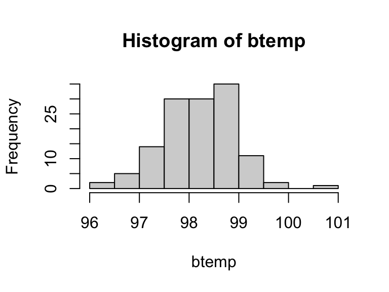
With \(n = 130\) and a clean, unimodal histogram, the t-test is appropriate here.
CautionYour turn 1 [L4]
Is the t-test appropriate for heart rate?
Extract heart.rate from temps and store a summary() of it as hrate.summary. Make a histogram and assess whether the t-test is appropriate.
TipSolution
# extract heart rate, summarize, and check the distribution
hrate <- temps$heart.rate
hrate.summary <- summary(hrate)
hrate.summary
Min. 1st Qu. Median Mean 3rd Qu. Max.
57.00 69.00 74.00 73.76 79.00 89.00 hist(hrate, breaks = 10)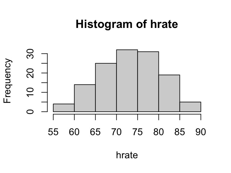
The distribution is unimodal with no extreme outliers or strong skewness. With \(n = 130\), the t-test is appropriate.
Specifying the null hypothesis
Is the mean body temperature really 98.6°F?
t.test(x, mu = ...) tests whether the population mean equals the value given by mu. The output reports the test statistic \(T\), degrees of freedom, \(p\)-value, and a 95% confidence interval.
# test whether mean body temperature equals 98.6°F
t.test(btemp, mu = 98.6)
    One Sample t-test

data:  btemp
t = -5.4548, df = 129, p-value = 2.411e-07
alternative hypothesis: true mean is not equal to 98.6
95 percent confidence interval:
 98.12200 98.37646
sample estimates:
mean of x
 98.24923
The \(p\)-value is far below 0.05. We report:
The data provide strong evidence that mean body temperature differs from 98.6°F (T = −5.45, df = 129, p < 0.0001).
CautionYour turn 2 [L4]
Is the mean resting heart rate 73 bpm?
Run t.test() on hrate with mu = 73 and store the result as hrate.tt. Interpret the result in one sentence.
TipSolution
# test whether mean heart rate equals 73 bpm
hrate.tt <- t.test(hrate, mu = 73)
hrate.tt
    One Sample t-test

data:  hrate
t = 1.2295, df = 129, p-value = 0.2211
alternative hypothesis: true mean is not equal to 73
95 percent confidence interval:
 72.53607 74.98701
sample estimates:
mean of x
 73.76154
The data do not provide evidence that mean heart rate differs from 73 bpm (T = 1.23, df = 129, p = 0.22).
Specifying the alternative
Was mean body temperature below 98.6°F?
The default alternative is two-sided. Use alternative = "less" or alternative = "greater" for a directional test.
# lower-sided: test whether mean body temp is less than 98.6°F
t.test(btemp, mu = 98.6, alternative = "less")
    One Sample t-test

data:  btemp
t = -5.4548, df = 129, p-value = 1.205e-07
alternative hypothesis: true mean is less than 98.6
95 percent confidence interval:
     -Inf 98.35577
sample estimates:
mean of x
 98.24923
# upper-sided: test whether mean body temp is greater than 98.6°F
t.test(btemp, mu = 98.6, alternative = "greater")
    One Sample t-test

data:  btemp
t = -5.4548, df = 129, p-value = 1
alternative hypothesis: true mean is greater than 98.6
95 percent confidence interval:
 98.14269      Inf
sample estimates:
mean of x
 98.24923
The lower-sided test gives a small \(p\)-value — the data clearly support \(\mu < 98.6\). The upper-sided test gives a \(p\)-value near 1, indicating no support for \(\mu > 98.6\). In each case the alternative hypothesis line in the output confirms what is being tested.
CautionYour turn 3 [L4]
A resting heart rate above 73 bpm may signal elevated cardiovascular stress. Is there evidence the mean exceeds 73?
Run the appropriate one-sided test and store the result as hrate.tt2. Interpret the result in one sentence.
TipSolution
# upper-sided: test whether mean heart rate exceeds 73 bpm
hrate.tt2 <- t.test(hrate, mu = 73, alternative = "greater")
hrate.tt2
    One Sample t-test

data:  hrate
t = 1.2295, df = 129, p-value = 0.1106
alternative hypothesis: true mean is greater than 73
95 percent confidence interval:
 72.73537      Inf
sample estimates:
mean of x
 73.76154
The data do not provide evidence that mean heart rate exceeds 73 bpm (T = 1.23, df = 129, p = 0.11).
Tests and intervals
What does the confidence interval tell us about hypothesis tests?
Run t.test(btemp) without a mu argument to get just the confidence interval:
# 95% confidence interval for mean body temperature
t.test(btemp)$conf.int
[1] 98.12200 98.37646
attr(,"conf.level")
[1] 0.95The 95% CI is approximately (98.12, 98.38). Now consider three candidate null values:
- \(\mu_0 = 98.25\) — inside the interval
- \(\mu_0 = 98.10\) — just outside the interval
- \(\mu_0 = 98.60\) — clearly outside the interval
CautionYour turn 4 [L4]
Before running any code, predict: which of the three null values above would be rejected by a two-sided test at \(\alpha = 0.05\)?
Then check your predictions by running t.test(btemp, mu = ...) for each value. Finally, write one sentence describing the general pattern you observe between the confidence interval and the test decisions.
TipSolution
# test each candidate null value
t.test(btemp, mu = 98.25)
    One Sample t-test

data:  btemp
t = -0.011962, df = 129, p-value = 0.9905
alternative hypothesis: true mean is not equal to 98.25
95 percent confidence interval:
 98.12200 98.37646
sample estimates:
mean of x
98.24923 t.test(btemp, mu = 98.10)
    One Sample t-test

data:  btemp
t = 2.3207, df = 129, p-value = 0.02187
alternative hypothesis: true mean is not equal to 98.1
95 percent confidence interval:
 98.12200 98.37646
sample estimates:
mean of x
98.24923 t.test(btemp, mu = 98.60)
    One Sample t-test

data:  btemp
t = -5.4548, df = 129, p-value = 2.411e-07
alternative hypothesis: true mean is not equal to 98.6
95 percent confidence interval:
 98.12200 98.37646
sample estimates:
mean of x
 98.24923
The test fails to reject \(\mu_0 = 98.25\) (\(p = 0.99\)) and rejects both \(\mu_0 = 98.10\) (\(p = 0.022\)) and \(\mu_0 = 98.60\) (\(p < 0.0001\)) — exactly matching which values fall inside vs. outside the 95% CI. The general pattern: the 95% confidence interval contains exactly the null values that a two-sided test would fail to reject at \(\alpha = 0.05\).
NoteSubmitting this assignment
- Save the file (Ctrl+S / Cmd+S).
- Render to PDF: click Render or press Ctrl+Shift+K / Cmd+Shift+K.
- Download both files: in the Files panel, check the
.qmdand PDF, then click More ▾ → Export…. - Upload the PDF to the Gradescope assignment for this lab.
- Upload the
.qmdfile to the course submission link.