Homework 2

With solutions

Author

Your Name Here

Before you begin

Fill in the author and calpoly-id fields at the very top of this file. Replace "Your Name Here" with your full name and "yourpolynetid" with your Cal Poly username (the part of your email before @calpoly.edu, e.g. jdoe01). Your submission cannot be matched to your record without this.

Where a problem asks you to save a result by a specific name (shown in bold), use the exact name given — your work is checked automatically.

Refer to Lab 4 for problem 1, Lab 5 for problems 2 and 3, and Lab 6 for problem 4.

Question 1: Hippocampal volume

Studies have provided evidence that the hippocampus is smaller in schizophrenic patients on average. The hippocampus dataset contains data on left hippocampal volume in cubic centimeters for pairs of monozygotic twins; one twin in each pair was affected by schizophrenia and the other was not. The difference variable records the difference in volume (unaffected − affected) within each pair.

# load data
load('data/hippocampus.RData')

Part a: Histogram [L3]

Construct a histogram of the differences in hippocampal volume. Are there any major outliers?

Solution

hist(hippocampus$difference)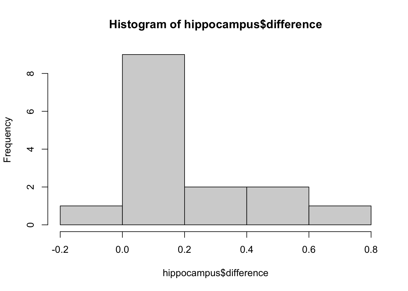

The histogram is shown above. There are no major outliers.

Part b: Two-sided test [L5]

Test whether mean hippocampal volume differs between affected and unaffected twins at the 1% significance level. Report the result in context following conventional style.

Solution

t.test(hippocampus$difference, alternative = 'two.sided', conf.level = 0.99)


    One Sample t-test

data:  hippocampus$difference
t = 3.2289, df = 14, p-value = 0.006062
alternative hypothesis: true mean is not equal to 0
99 percent confidence interval:
 0.01551009 0.38182325
sample estimates:
mean of x 
0.1986667

The data provide evidence that mean hippocampal volume differs between affected and unaffected twins (T = 3.229 on 14 df, p = 0.006).

Part c: One-sided test [L5]

Test whether mean hippocampal volume is greater among unaffected twins compared with their affected co-twins at the 1% significance level. Report the result in context following conventional style.

Solution

t.test(hippocampus$difference, alternative = 'greater', conf.level = 0.99)


    One Sample t-test

data:  hippocampus$difference
t = 3.2289, df = 14, p-value = 0.003031
alternative hypothesis: true mean is greater than 0
99 percent confidence interval:
 0.03718909        Inf
sample estimates:
mean of x 
0.1986667

The data provide evidence that mean hippocampal volume is greater among unaffected individuals than their affected co-twins (T = 3.229 on 14 df, p = 0.003).

Part d: Confidence bound [L5]

Construct a lower 99% confidence bound for the mean difference in hippocampal volume (unaffected − affected). Interpret the result in context following conventional style.

Solution

The lower bound is given directly by the confidence interval from part (c). With 99% confidence, the mean hippocampal volume of unaffected twins is estimated to be at least 0.037 cm³ greater than that of their affected co-twins.

Question 2: Frog egg clutches

Note: parts (a) through (d) should be done entirely by hand based on the figures and table below. Type your solutions in the space provided.

Chen, W., et al., Maternal investment increases with altitude in a frog on the Tibetan Plateau. Journal of Evolutionary Biology 26-12 (2013) reported measurements of egg clutch sizes for frogs at breeding ponds in the eastern Tibetan Plateau. The figures and summary table below show clutch size distributions for two sites.

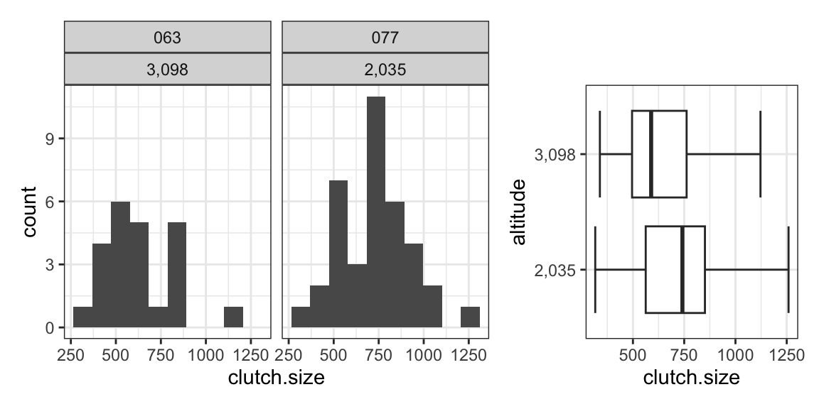
site	altitude	csize.mean	csize.sd	n
063	3,098	625.67	197.01	23
077	2,035	733.44	202.72	37

Part a: Point estimate and SE [L4]

Compute a point estimate and standard error for the difference in mean clutch size between the two sites (site 077 − site 063). Report these quantities in context following conventional style.

Solution

\[\hat{\mu}_{077} - \hat{\mu}_{063} = 733.44 - 625.67 = 107.77\]

\[SE = \sqrt{\frac{197.01^2}{23} + \frac{202.72^2}{37}} = \sqrt{1686.6 + 1111.5} = \sqrt{2798.1} \approx 52.9\]

The difference in mean clutch size (site 077 − site 063) is estimated to be 107.8 eggs (SE = 52.9).

Part b: 99% confidence interval [L4]

Construct an approximate 99% confidence interval for the difference in mean clutch size and interpret the result in context following conventional style.

Solution

\[107.77 \pm 3 \times 52.9 = 107.77 \pm 158.7 = (-50.9,\ 266.5)\]

With 99% confidence, the difference in mean clutch size (site 077 − site 063) is estimated to be between −50.9 and 266.5 eggs.

Part c: Test statistic [L5]

Compute the test statistic for a test of whether mean clutch size differs between the two sites.

Solution

\[T = \frac{\hat{\mu}_{077} - \hat{\mu}_{063}}{SE} = \frac{107.77}{52.9} = 2.037\]

Part d: Conclusion [L5]

What would the conclusion of the test be at the 1% significance level? Explain your reasoning.

Solution

At the 1% level, there is not sufficient evidence of a difference in mean clutch size between the two sites. The 99% interval from part (b) includes zero (so no difference is plausible at the corresponding confidence level), or equivalently \(|T| = 2.037 \ll 3\).

Question 3: Lizard running speed

The lizards dataset contains top running speeds (m/s) for two species: western fence lizard and sagebrush lizard.

# load data
load('data/lizards.RData')

Part a: Boxplots [L3]

Construct side-by-side boxplots of top running speed by species. Does there appear to be a difference in mean speed between species? If so, which species appears to run faster?

Solution

boxplot(top.speed ~ species, data = lizards, horizontal = TRUE)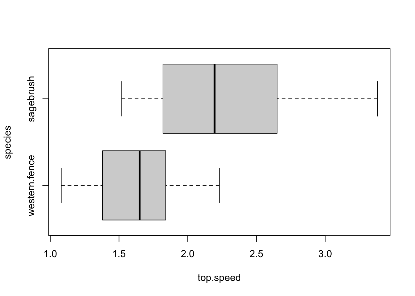

Sagebrush lizards appear to run faster on average than western fence lizards.

Part b: Two-sample t-test [L5]

Test for a difference in mean top running speed between species at the 5% significance level. Store the p-value as lizard.pval. Report the test result following conventional style.

Solution

tt.out      <- t.test(top.speed ~ species, data = lizards)
lizard.pval <- tt.out$p.value
tt.out


    Welch Two Sample t-test

data:  top.speed by species
t = -5.2217, df = 32.57, p-value = 9.939e-06
alternative hypothesis: true difference in means between group western.fence and group sagebrush is not equal to 0
95 percent confidence interval:
 -0.9754526 -0.4282537
sample estimates:
mean in group western.fence     mean in group sagebrush 
                   1.612692                    2.314545

The data provide evidence of a difference in mean top running speed between western fence and sagebrush lizards (T = −5.222 on 32.57 df, p < 0.0001).

Part c: Point estimate and SE [L4]

Report a point estimate and standard error for the difference in mean top running speed following conventional style.

Solution

c(diff = diff(tt.out$estimate), se = tt.out$stderr)

diff.mean in group sagebrush                           se 
                   0.7018531                    0.1344115

The mean top running speed of sagebrush lizards is estimated to be 0.702 m/s faster than that of western fence lizards (SE 0.134).

Part d: Confidence interval [L4]

Construct a confidence interval at a level consistent with your test in part (b) and interpret the interval in context following conventional style.

Solution

tt.out$conf.int

[1] -0.9754526 -0.4282537
attr(,"conf.level")
[1] 0.95

With 95% confidence, the mean top running speed of sagebrush lizards is estimated to be between 0.428 and 0.976 m/s faster than that of western fence lizards.

Part e: Sample size [L5]

How many lizards of each species would you need to measure to detect a difference in mean top speed of 0.5 m/s using the test above 85% of the time? Use the larger of the two sample standard deviations to perform the calculation.

Solution

# find the larger SD
max.sd <- max(tapply(lizards$top.speed, lizards$species, sd))
max.sd

[1] 0.5554983

# sample size calculation
power.t.test(delta       = 0.5,
             sd          = max.sd,
             type        = 'two.sample',
             alternative = 'two.sided',
             sig.level   = 0.05,
             power       = 0.85)


     Two-sample t test power calculation 

              n = 23.16644
          delta = 0.5
             sd = 0.5554983
      sig.level = 0.05
          power = 0.85
    alternative = two.sided

NOTE: n is number in *each* group

You would need 24 lizards per species (48 total).

Question 4: Meadowfoam

Meadowfoam is a small plant found in moist meadows of the US Pacific Northwest. Researchers investigated the effect of light intensity (μmol/m²/sec) on flowering in a controlled growth chamber by recording the average number of flowers per plant in experimental plots exposed to one of six intensity levels. The data are stored in the meadow dataset.

library(effectsize)
load('data/meadow.RData')

Part a: Boxplots [L3]

Construct side-by-side boxplots of flowers per plant by intensity level. Does it appear that mean flowering varies by light intensity? If so, describe the apparent relationship.

Solution

boxplot(flowers ~ intensity, data = meadow, xlab = 'light intensity (μmol/m²/sec)')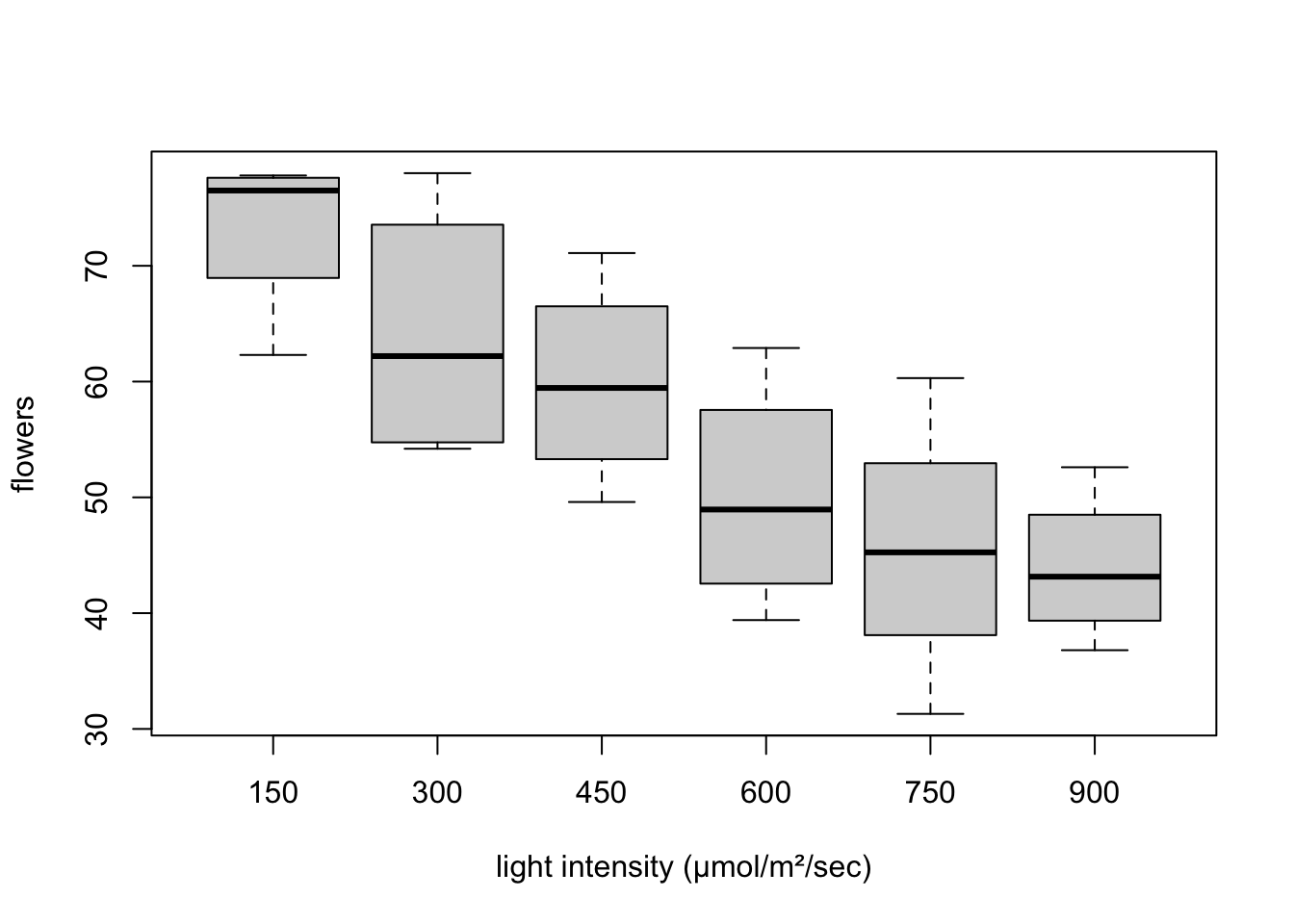

Mean flowering does appear to vary by light intensity: the number of flowers per plant tends to decrease as light intensity increases.

Part b: Assumptions [L9]

Do the data appear to satisfy the assumptions for ANOVA? Explain.

Solution

Yes. Variation in flowering is similar across intensity levels and there are no major outliers, so the equal-variance and no-outliers assumptions appear satisfied.

Part c: Omnibus test [L9]

Test for an effect of light intensity on mean flowering at the 1% significance level. Store the fitted model as fit. Report the result of the omnibus test in context following conventional style.

Solution

fit <- aov(flowers ~ intensity, data = meadow)
summary(fit)

            Df Sum Sq Mean Sq F value  Pr(>F)   
intensity    5   2684   536.7   5.839 0.00224 **
Residuals   18   1654    91.9                   
---
Signif. codes:  0 '***' 0.001 '**' 0.01 '*' 0.05 '.' 0.1 ' ' 1

The data provide evidence of an effect of light intensity on mean flowering (F = 5.839 on 5 and 18 df, p = 0.002).

Part d: Effect size [L9]

Estimate the effect size \(\eta^2\) with a 99% confidence interval. Interpret the interval in context following conventional style.

Solution

eta_squared(fit, partial = FALSE, alternative = 'two.sided', ci = 0.99)

# Effect Size for ANOVA (Type I)

Parameter | Eta2 |       99% CI
-------------------------------
intensity | 0.62 | [0.05, 0.80]

An estimated 62% of variation in flowering is attributable to light intensity. With 99% confidence, an estimated 5%–80% of variation in flowering is attributable to light intensity.

Part e: Unexplained variation [L9]

Estimate the proportion of variation in flowering not attributable to light intensity.

Solution

If an estimated 62% of variation in flowering is attributable to light intensity, then the estimated proportion not attributable is \(1 - 0.62 = 0.38\), or 38%.

Submitting this assignment

Save the file (Ctrl+S / Cmd+S).
Render to PDF: click Render or press Ctrl+Shift+K / Cmd+Shift+K.
Download both files: in the Files panel, check the .qmd and PDF, then click More ▾ → Export….
Upload the PDF to the Gradescope assignment for this homework.
Upload the .qmd file through the submission link on the course page.