Homework 1

With solutions

Author

Your Name Here

Before you begin

Fill in the author and calpoly-id fields at the very top of this file. Replace "Your Name Here" with your full name and "yourpolynetid" with your Cal Poly username (the part of your email before @calpoly.edu, e.g. jdoe01). Your submission cannot be matched to your record without this.

Where a problem asks you to save a result by a specific name (shown in bold), use the exact name given — your work is checked automatically.

Refer to Lab 2 for problems 1 and 2, and Lab 3 for problems 3 and 4.

Question 1: Census data

The census dataset contains a sample of responses from the 2000 U.S. census.

# load census data
load('data/census.RData')

Part a: Number of variables [L1]

How many variables are in the dataset, not including census year and FIPS code?

Solution

There are 8 columns in the dataframe, so not including year and FIPS, there are 6 variables.

Part b: Categorical variables [L1]

How many categorical variables are in the dataset, not including FIPS code?

Solution

Not including FIPS, there are 3 categorical variables: sex, race_general, and marital_status.

Part c: Sample size [L1]

How many respondents are included in the dataset?

Solution

There are 377 individuals in the sample (one per row).

Part d: Age range [L3]

What are the ages of the youngest and oldest individuals in the sample?

Solution

# extract age and find the range
age <- census$age
min(age)

[1] 15

max(age)

[1] 93

The minimum and maximum ages are shown in the output above.

Part e: Income histogram [L3]

Construct a histogram of total family incomes with an appropriate amount of binning.

Solution

# extract total family income and plot
family.income <- census$total_family_income
hist(family.income, breaks = 50)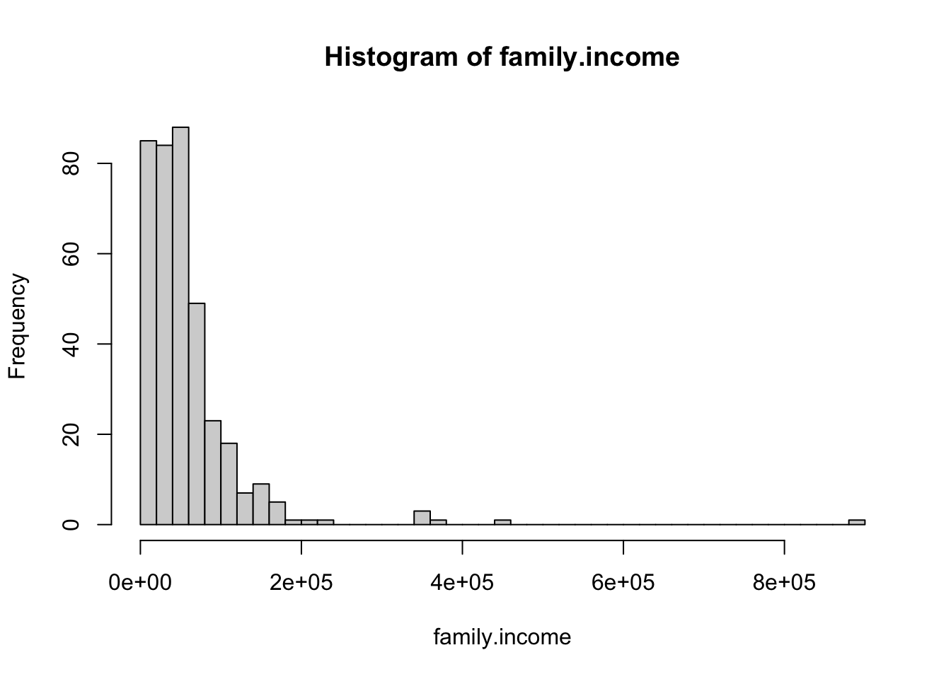

Around 50 bins captures the shape well.

Part f: Center and spread [L3]

Determine and compute appropriate measures of center and spread for total family income.

Solution

# median and IQR are appropriate for a right-skewed distribution
median(family.income)

[1] 44000

IQR(family.income)

[1] 48000

The incomes are heavily right-skewed with some large outliers, so median and IQR are better choices than mean and SD. The median family income is $44K; the IQR is $48K.

Question 2: NHANES data

The nhanes dataset contains responses from the National Health and Nutrition Examination Survey (NHANES) on a subset of demographic and health-related variables. Assume that respondents are a representative sample of U.S. adults.

# load NHANES data
load('data/nhanes.RData')

Part a: Variable types [L1]

Which variables are numeric and which are categorical?

Solution

All variables are numeric except for gender.

Part b: Discrete or continuous [L1]

Classify each numeric variable as discrete or continuous.

Solution

All variables are discrete (integer-valued) except for totchol.

Part c: Dataset dimensions [L1]

How many observations and variables are in the dataset?

Solution

There are 3179 observations of 8 variables.

Part d: Proportion male [L3]

What proportion of respondents are male?

Solution

# count respondents by gender and convert to proportions
table(nhanes$gender) |> proportions()


   female      male 
0.4995282 0.5004718

50.05% of respondents were male.

Part e: Blood pressure distributions [L3]

Make histograms of systolic and diastolic blood pressure (bpsys1 and bpdia1, respectively). Describe the distributions.

Solution

# histogram of systolic blood pressure
hist(nhanes$bpsys1)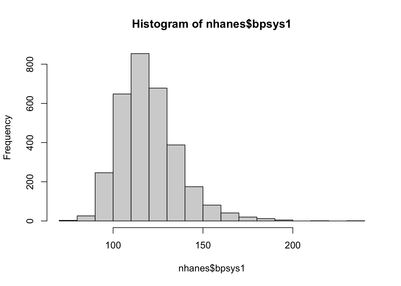

# histogram of diastolic blood pressure
hist(nhanes$bpdia1)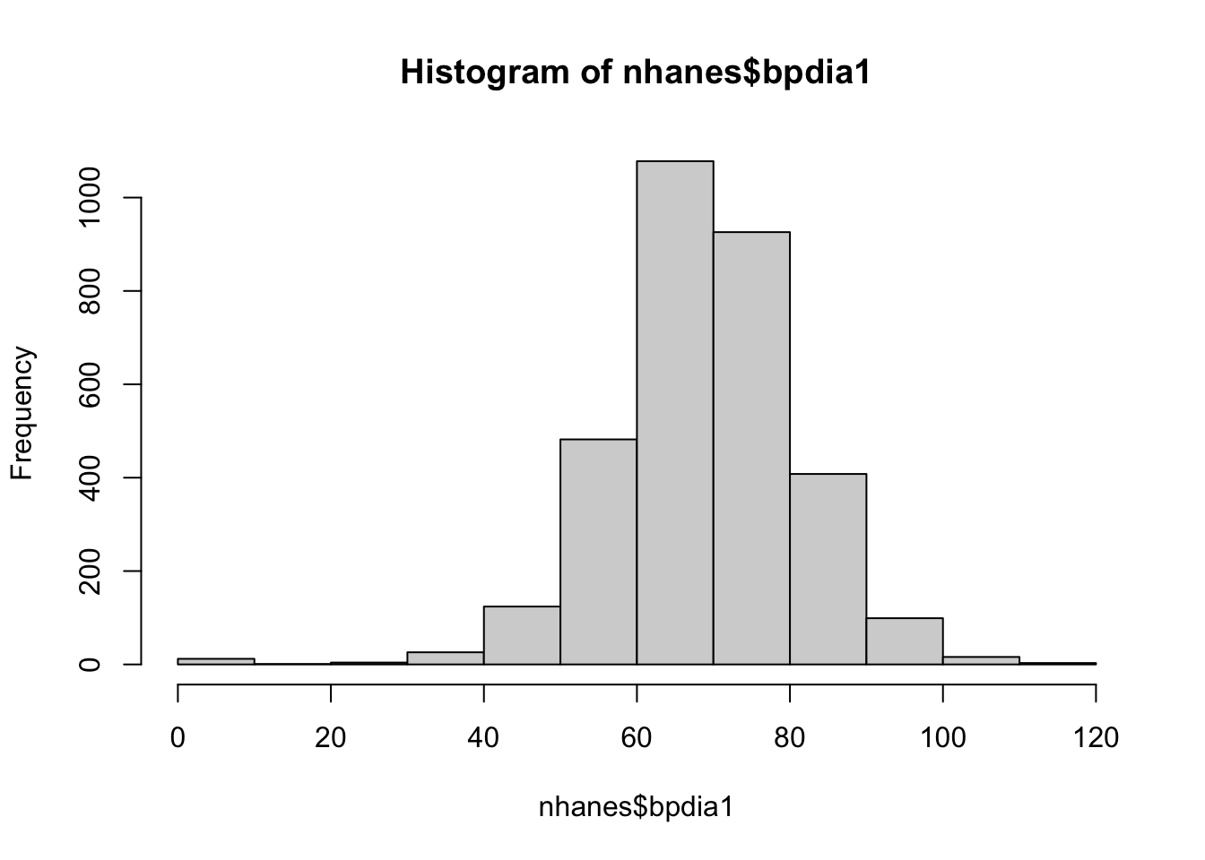

The distribution of systolic pressure is right-skewed, and the distribution of diastolic pressure is roughly symmetric. Both are unimodal.

Part f: Hypertension count [LX]

A person is considered to have hypertension if their systolic pressure is over 130 OR their diastolic pressure is over 80. How many individuals in the dataset have hypertension? (Hint: sum(x > 5) will calculate how many values in x exceed 5.)

Solution

# flag individuals exceeding each threshold, then count those meeting either condition
sys.over130 <- nhanes$bpsys1 > 130
dia.over80  <- nhanes$bpdia1 > 80
sum(sys.over130 | dia.over80)

[1] 1010

1010 individuals, approximately one third of respondents, have hypertension.

Question 3: Frog data

Chen, W., et al., Maternal investment increases with altitude in a frog on the Tibetan Plateau. Journal of Evolutionary Biology 26-12 (2013) includes an analysis of measurements pertaining to egg clutches of several frog populations at breeding ponds (sites) in the eastern Tibetan Plateau: egg size (diameter in mm), clutch size (estimated number of eggs), clutch volume (volume in cubic mm), and body size (length of mother in cm). The frog dataset contains an excerpt of data from this paper along with a study site identifier and site altitude.

# load frog data
load('data/frog.RData')

Part a: Observations by site [L1]

Which site has the most observations? The least?

Solution

# tally observations per site
table(frog$site)


019 030 040 053 060 063 069 077 105 109 118 
 10   6 172   6  10  23  14  37 127  21   5

Site 118 has the fewest observations (5); site 040 has the most (172).

Part b: Altitude variable type [L1]

Notice that altitude is recorded as a categorical variable. What type of categorical variable is it, and what about the study might explain why it is recorded this way rather than as numeric?

Solution

Altitude is ordinal. It is recorded this way because each site is associated with exactly one altitude, so there are only 11 unique values, each occurring multiple times. Moreover, since the spacing between observed altitudes is irregular, it is more sensible to treat altitude as ordinal than as discrete numeric.

Part c: Clutch size distribution [L3]

Make a histogram of clutch size and describe the distribution.

Solution

# histogram of clutch size
hist(frog$clutch.size, breaks = 15)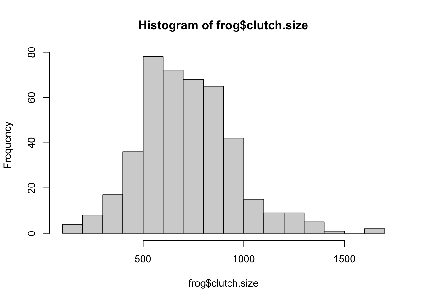

Clutch size is unimodal and slightly right-skewed.

Part d: Summary statistics [L3]

Compute summary statistics of clutch size via summary(). Choose an appropriate measure of center.

Solution

# five-number summary and mean for clutch size
summary(frog$clutch.size)

   Min. 1st Qu.  Median    Mean 3rd Qu.    Max. 
  158.5   549.5   707.9   721.3   851.1  1698.2

The distribution is not severely skewed and has no extreme outliers, so mean and median are both reasonable choices.

Part e: Point estimate and SE [L4]

Use the data to estimate mean clutch size; report the point estimate and standard error following conventional style. Store the t.test() result as clutchsize.tt.

Solution

# run t.test and retrieve point estimate and standard error
clutchsize.tt <- t.test(frog$clutch.size)
clutchsize.tt$estimate

mean of x 
 721.2504

clutchsize.tt$stderr

[1] 11.41506

Mean clutch size is estimated to be 721.25 eggs (SE 11.42).

Part f: 99% confidence interval [L4]

Construct a 99% confidence interval for mean clutch size and interpret the result in context following conventional style.

Solution

# 99% confidence interval for mean clutch size
t.test(frog$clutch.size, conf.level = 0.99)$conf.int

[1] 691.7161 750.7847
attr(,"conf.level")
[1] 0.99

With 99% confidence, the mean clutch size is estimated to be between 691.7 and 750.8 eggs.

Part g: Unusual clutch size [L3]

Would a clutch size of 200 be unusual? Explain.

Solution

# check where 200 falls relative to the distribution
summary(frog$clutch.size)

   Min. 1st Qu.  Median    Mean 3rd Qu.    Max. 
  158.5   549.5   707.9   721.3   851.1  1698.2

quantile(frog$clutch.size, probs = 0.01)

      1% 
237.7373

Yes, a clutch size of 200 would be unusually small. The 1st percentile is 237.7, so more than 99% of observed clutches are larger than 200.

Question 4: Nests

Note: parts (a) through (d) should be done entirely by hand based on the textbook exercise. Type your solutions in the space below each part.

Part a: Point estimate of mean [L4]

Estimate the population mean BGC of nests.

Solution

The population mean BGC of nests is estimated to be 0.6052.

Part b: Point estimate of SD [L4]

Estimate the population standard deviation of BGC of nests.

Solution

The population standard deviation of BGC of nests is estimated to be 0.0131.

Part c: Standardized value [L4]

Would a BGC value of 0.63 be unusual?

Solution

A BGC value of 0.63 would be somewhat high but not extreme — it is 1.9 standard errors above the sample mean.

Part d: Interval by hand [L4]

Construct an interval estimate for the mean BGC of nests.

Solution

The mean BGC of nests is estimated to be between 0.6021 and 0.6083 units.

Part e: 95% CI using the empirical rule [L4]

Compute a 95% confidence interval for the mean BGC of nests using the empirical rule and interpret the interval in context following conventional style.

Solution

Using $c = 2$: $0.6052 \pm 2 \times SE$. With the SE from part (b) and the sample size given in the textbook, this yields an interval consistent with part (d). With 95% confidence, the mean BGC of nests is estimated to be between 0.6021 and 0.6083 units.

Part f: Effect of sample size [L4]

Supposing a sample of 30 nests returned exactly the same summary statistics, recompute your interval from part (e). Is the margin of error smaller or larger?

Solution

With a smaller sample size ($n = 30$ instead of the original $n$), the standard error increases, so the margin of error is larger and the interval is wider.

Submitting this assignment

Save the file (Ctrl+S / Cmd+S).
Render to PDF: click Render or press Ctrl+Shift+K / Cmd+Shift+K.
Download both files: in the Files panel, check the .qmd and PDF, then click More ▾ → Export….
Upload the PDF to the Gradescope assignment for this homework.
Upload the .qmd file through the submission link on the course page.