Applied Statistics for Life Sciences
In STAT218 we cover statistical inference for:
But the basic framework generalizes quite broadly.

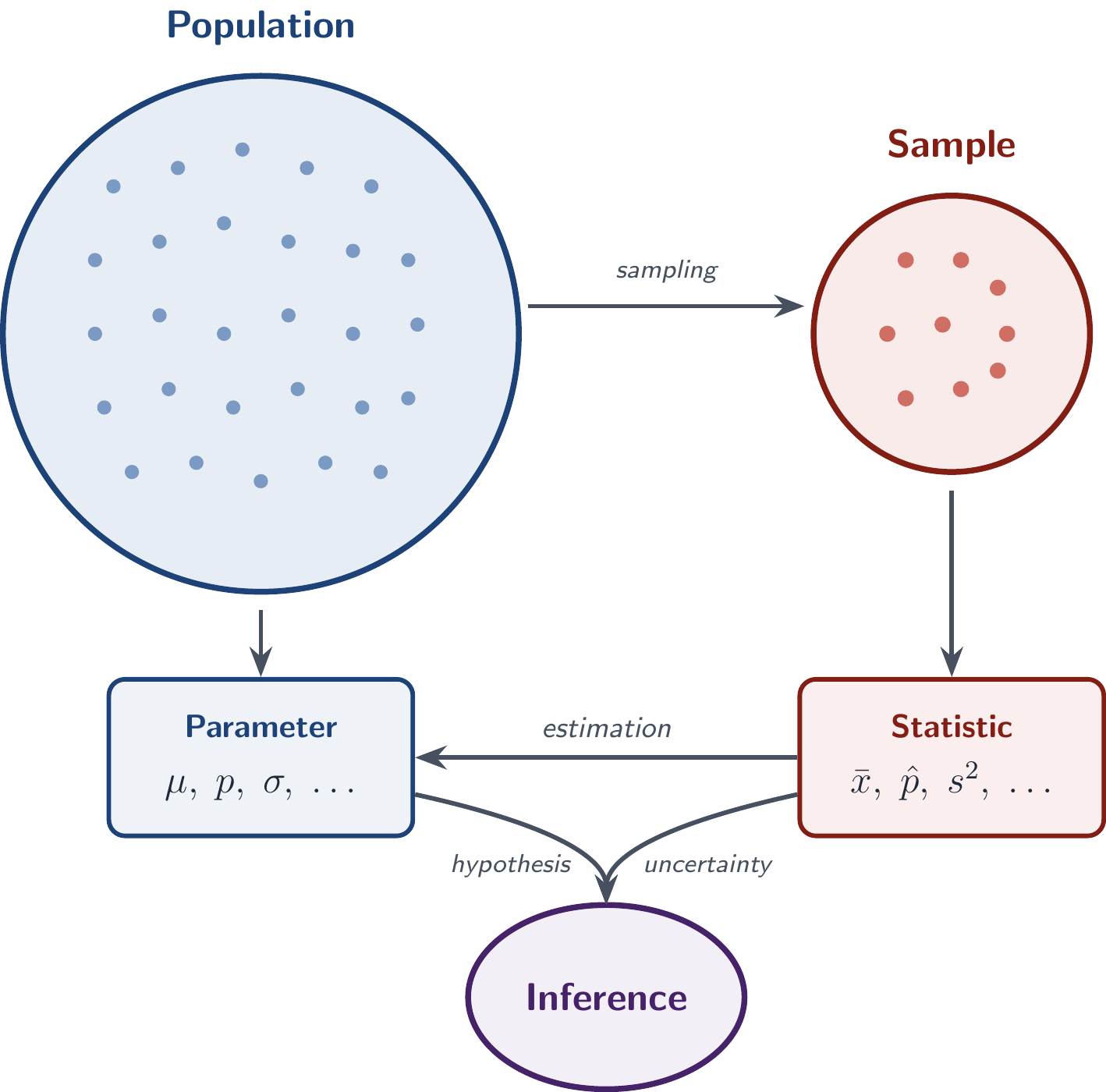
Every method in this course follows the same logical template:
What changes from method to method is what fills each slot — the logic stays the same.
Almost every result in this course can be reported in one of two forms:
Test result:
The data provide [evidence / no evidence] that [claim about parameter].
Interval estimate:
With 95% confidence, [parameter] is estimated to be between [lower] and [upper].
Data: \(n\) measurements of a continuous variable.
Parameter: population mean \(\mu\)
Hypotheses: \(\quad\begin{cases} H_0: \mu = \mu_0 \\ H_A: \mu \neq \mu_0 \quad\text{(or } <, > \text{)} \end{cases}\)
Test statistic: \(\quad T = \dfrac{\bar{x} - \mu_0}{SE(\bar{x})} \quad\text{where}\quad SE(\bar{x}) = \dfrac{s_x}{\sqrt{n}}\)
Sampling distribution: \(\quad t_{n - 1}\) model
Confidence interval: \(\quad \bar{x} \pm c \times SE(\bar{x})\)
Assumptions: observations are independent; underlying distribution is approximately normal (robust for large \(n\)).
Is the true mean body temperature actually 98.6°F?
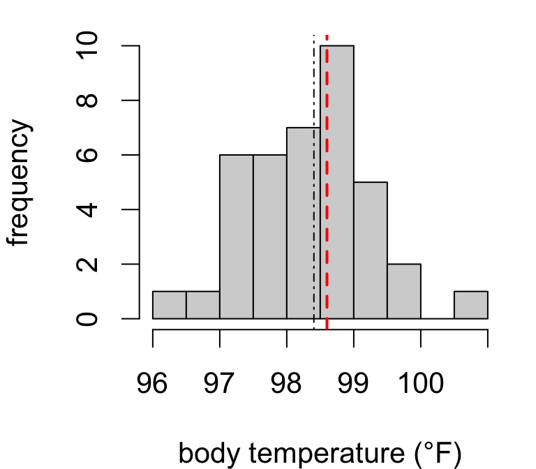
The data provide evidence that mean body temperature differs from 98.6°F (T = -2.24 on 129 degrees of freedom, p = 0.027). With 95% confidence, the mean is estimated to be between 98.12 and 98.57°F.
Do U.S. adults sleep an average of 8 hours per night? (NHANES data)
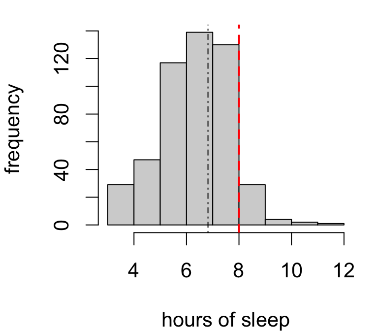
The data provide evidence that the average U.S. adult does not sleep 8 hours per night (T = -42.53 on 3178 degrees of freedom, p < 0.0001). With 95% confidence, the mean nightly hours of sleep among U.S. adults is estimated to be between 6.91 and 7.01 hours.
Data: measurements of a continuous variable from two groups (paired or independent).
Testing a mean difference (paired data): inference on \(\delta = \mu_\text{before} - \mu_\text{after}\) or similar.
Testing a difference in means (independent samples): inference on \(\mu_1 - \mu_2\).
Test statistic: \(\quad T = \dfrac{\bar{x} - \bar{y}}{SE(\bar{x} - \bar{y})} \quad\text{where}\quad SE = \sqrt{\dfrac{s_x^2}{n_x} + \dfrac{s_y^2}{n_y}}\)
Sampling distribution: \(\quad t_\nu\) model
Confidence interval: \(\quad (\bar{x} - \bar{y}) \pm c \times SE(\bar{x} - \bar{y})\)
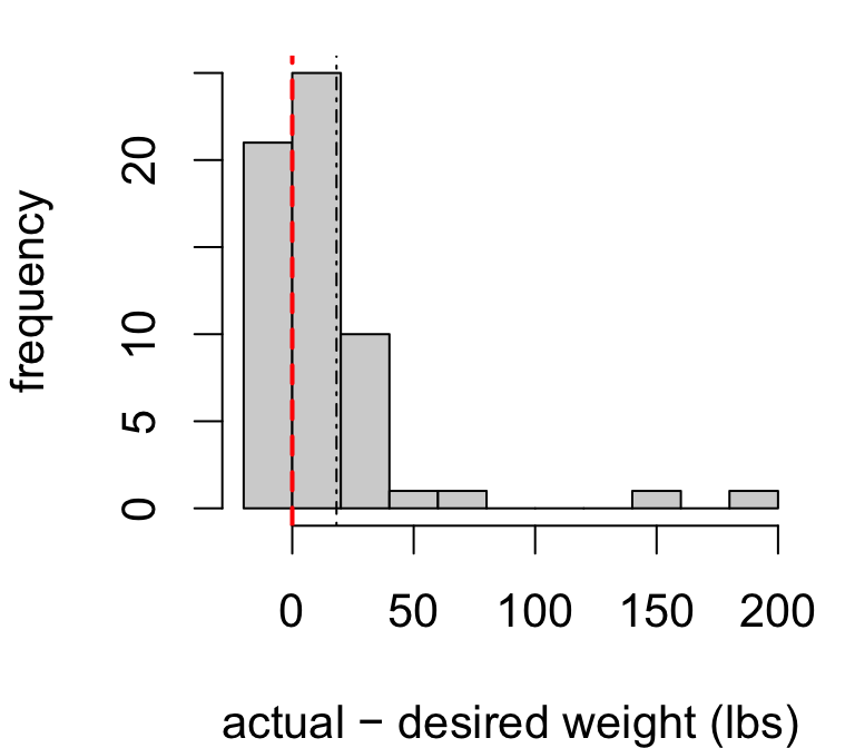
Does the average U.S. adult wish to lose weight?
One Sample t-test
data: weight.diffs
t = 4.2172, df = 59, p-value = 4.311e-05
alternative hypothesis: true mean is greater than 0
95 percent confidence interval:
10.99824 Inf
sample estimates:
mean of x
18.21667
The data provide evidence that the average U.S. adult’s actual weight exceeds their desired weight (T = 4.2172 on 59 degrees of freedom, p < 0.0001).
Did beak depth increase after the 1977 drought on Daphne Major?
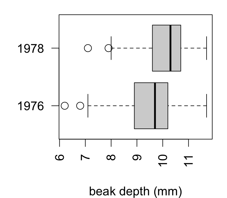
Welch Two Sample t-test
data: depth by year
t = -4.5833, df = 172.98, p-value = 4.37e-06
alternative hypothesis: true difference in means between group 1976 and group 1978 is less than 0
95 percent confidence interval:
-Inf -0.427321
sample estimates:
mean in group 1976 mean in group 1978
9.469663 10.138202
The data provide evidence that mean beak depth increased following the drought (T = -4.57 on 111.79 degrees of freedom, p < 0.0001).
Data: measurements of a continuous variable across \(k > 2\) groups.
Parameter: group means \(\mu_1, \dots, \mu_k\)
Hypotheses: \(\quad\begin{cases} H_0: \mu_1 = \mu_2 = \cdots = \mu_k \\ H_A: \text{at least two means differ} \end{cases}\)
Test statistic: \(\quad F = \dfrac{MSG}{MSE} \quad \left(\frac{\text{group variation}}{\text{individual variation}}\right)\)
Sampling distribution: \(\quad F_{k - 1,\; n - k}\) model
Effect size: \(\quad \eta^2 = \dfrac{SSG}{SSG + SST} \quad \left(\frac{\text{group variation}}{\text{total variation}}\right)\)
Post-hoc: pairwise contrasts \(\mu_i - \mu_j\) with multiple testing adjustment.
| Source | degrees of freedom | Sum of squares | Mean square | F statistic | p-value |
|---|---|---|---|---|---|
| Group | \(k - 1\) | SSG | \(MSG = \frac{SSG}{k - 1}\) | \(\frac{MSG}{MSE}\) | \(P(F > F_\text{obs})\) |
| Error | \(n - k\) | SSE | \(MSE = \frac{SSE}{n - k}\) |
Formally, the ANOVA model says \[\underbrace{(n - 1)S^2}_{SST} = SSG + SSE\]
Does caloric restriction affect mean lifespan in mice?
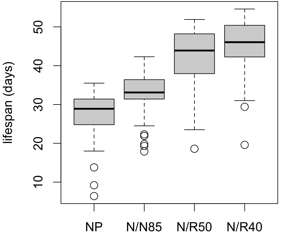
Df Sum Sq Mean Sq F value Pr(>F)
diet 3 11426 3809 87.41 <2e-16 ***
Residuals 233 10152 44
---
Signif. codes: 0 '***' 0.001 '**' 0.01 '*' 0.05 '.' 0.1 ' ' 1
The data provide evidence that diet restriction has an effect on mean lifetime among mice (F = 87.41 on 3 and 233 degrees of freedom, p < 0.0001). With 95% confidence, the proportion of variation in lifespan explained by diet is estimated to be between 44% and 60%.
Which diets differ? Pairwise contrasts with Bonferroni correction:
contrast estimate SE df t.ratio p.value
NP - (N/N85) -5.29 1.29 233 -4.113 0.0003
NP - (N/R50) -14.90 1.23 233 -12.150 <0.0001
NP - (N/R40) -17.71 1.27 233 -13.938 <0.0001
(N/N85) - (N/R50) -9.61 1.17 233 -8.183 <0.0001
(N/N85) - (N/R40) -12.43 1.22 233 -10.177 <0.0001
(N/R50) - (N/R40) -2.82 1.16 233 -2.436 0.0937
P value adjustment: bonferroni method for 6 tests
The data provide evidence at the 5% significance level that mean lifespan differs among all levels of diet restriction except the N/R40 and N/R50 groups (p = 0.0937), for which the evidence is suggestive but inconclusive.
Data: same setups as above, but assumptions are questionable (skew, outliers, small \(n\)).
| Parametric method | Nonparametric alternative |
|---|---|
| One-sample \(t\) test | Sign test, signed rank test |
| Two-sample \(t\) test | Wilcoxon rank sum test |
| ANOVA | Kruskal-Wallis test |
Parameter: population center (median or location)
Test statistic: varies (based on observation ordering)
Sampling distribution: via combinatorics
Nonparametrics are robust to non-normal data, but less powerful than parametric tests.
Does the median DDT concentration in kale exceed the 3ppm safety threshold?
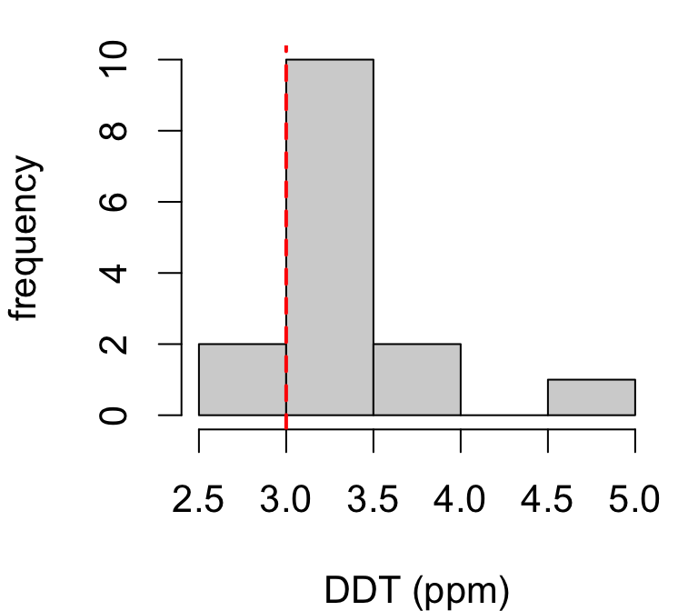
The data provide evidence that median DDT in kale exceeds 3ppm (p = 0.019).
Is there a difference in serum cholesterol between corn flake and oat bran diets?
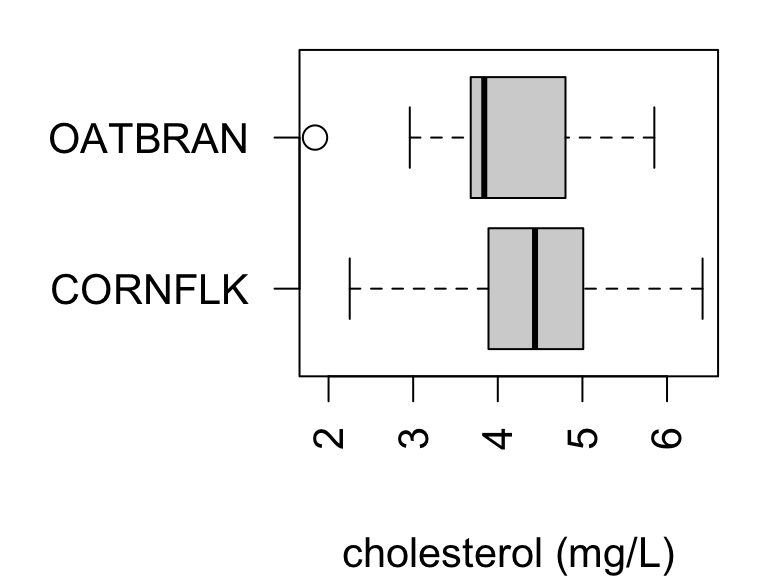
The data provide no evidence of a difference in cholesterol between diets (rank sum test, p = 0.74).
Does the distribution of AAM lengths differ by geographic location?
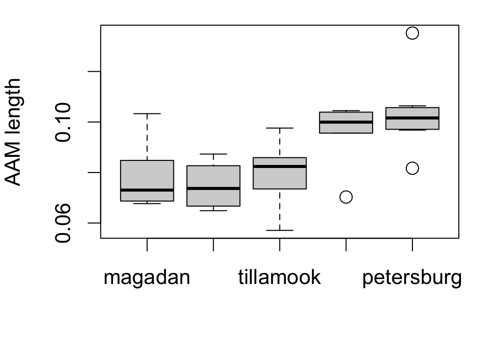
The data provide evidence that the distribution of AAM lengths differs by geographic location (Kruskal-Wallis test, p = 0.0025).
Data: paired measurements of two continuous variables (one response, one explanatory).
Model: \(\quad y = \beta_0 + \beta_1 x + \epsilon\)
Parameters: intercept \(\beta_0\), slope \(\beta_1\)
Inference for the slope:
\[ \begin{cases} H_0: &\beta_1 = 0 \quad\text{(no association)} \\ H_A: &\beta_1 \neq 0 \end{cases} \qquad T = \frac{\hat\beta_1}{SE(\hat\beta_1)} \sim t_{n - 2} \]
Predictions:
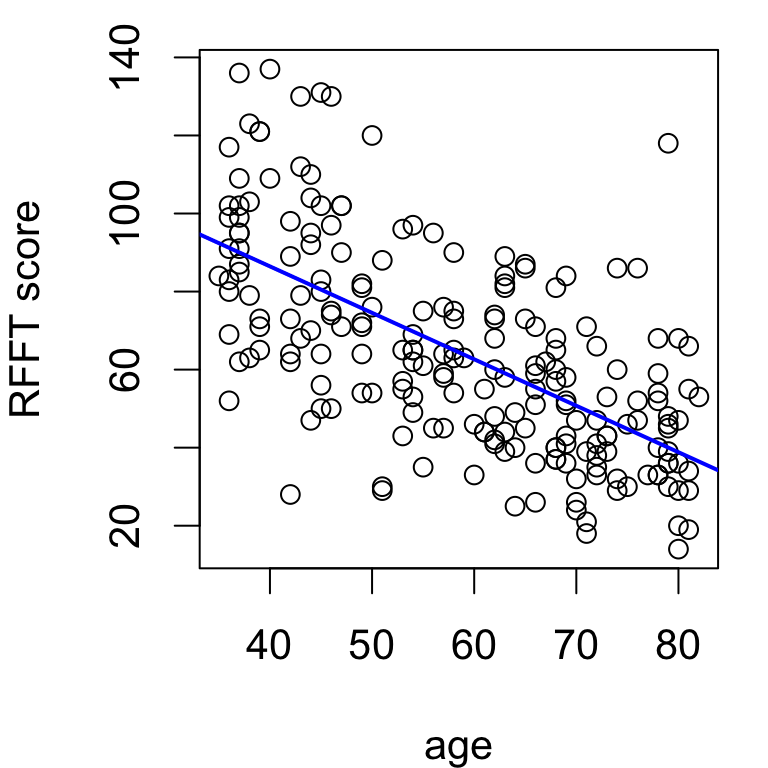
How much does RFFT score decline with age? (PREVEND data)
Call:
lm(formula = rfft ~ age, data = prevend)
Residuals:
Min 1Q Median 3Q Max
-56.085 -14.690 -2.937 12.744 77.975
Coefficients:
Estimate Std. Error t value Pr(>|t|)
(Intercept) 134.0981 6.0701 22.09 <2e-16 ***
age -1.1908 0.1007 -11.82 <2e-16 ***
---
Signif. codes: 0 '***' 0.001 '**' 0.01 '*' 0.05 '.' 0.1 ' ' 1
Residual standard error: 20.52 on 206 degrees of freedom
Multiple R-squared: 0.4043, Adjusted R-squared: 0.4014
F-statistic: 139.8 on 1 and 206 DF, p-value: < 2.2e-16
With each additional year of age, mean RFFT score decreases by an estimated 1.19 points.
With 95% confidence, each additional year of age is associated with a decrease in mean RFFT score of between 0.99 and 1.39 points.
fit lwr upr
1 68.60439 28.04903 109.1598
With 95% confidence, the RFFT score for an individual 55 year old is estimated to be between 28 and 109.2 points.
Data: \(n\) observations of a categorical variable with \(k\) categories.
Parameter: population proportions \(\mathbf{p} = (p_1, \dots, p_k)\)
Test statistic: \(\quad \chi^2 = \sum_i \dfrac{(O_i - E_i)^2}{E_i}\)
where \(O_i\) = observed count and \(E_i\) = expected count under \(H_0: \mathbf{p} = \mathbf{p}_0\).
Sampling distribution: \(\quad \chi^2_{k - 1}\) model
Confidence interval for \(p_k\): \(\quad \hat{p}_k \pm c \times \sqrt{\dfrac{\hat{p}_k(1 - \hat{p}_k)}{n}}\)
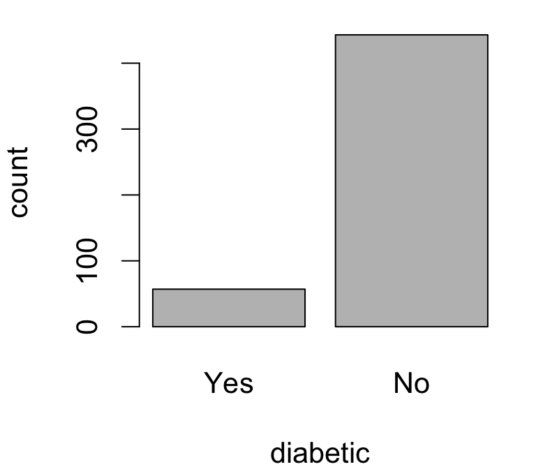
Is diabetes prevalence in the U.S. equal to 10%?
1-sample proportions test with continuity correction
data: 57 out of 500, null probability 0.1
X-squared = 0.93889, df = 1, p-value = 0.3326
alternative hypothesis: true p is not equal to 0.1
95 percent confidence interval:
0.08814952 0.14594579
sample estimates:
p
0.114
The data provide no evidence that diabetes prevalence differs from 10% (\(\chi^2\) = 0.94 on 1 degree of freedom, p = 0.33). With 95% confidence, diabetes prevalence among U.S. adults is estimated to be between 8.8% and 14.6%.
Data: \(J\) groups of \(n_j\) observations of a categorical variable with \(k\) categories.
Parameter: group/sample proportions \(\mathbf{p}_1, \dots, \mathbf{p}_J\)
Test statistic: \(\quad \chi^2 = \sum_{i, j} \dfrac{(O_{ij} - E_{ij})^2}{E_{ij}}\)
where \(O\) = observed count, \(E\) = expected count under \(H_0: \mathbf{p}_1 = \cdots = \mathbf{p}_J\)
Residuals explain where an association/difference lies: \(\quad r_{ij} = \dfrac{O_{ij} - E_{ij}}{\sqrt{E_{ij}}}\)
Measures of association for \(2 \times 2\) tables:
Do ACTN3 genotype frequencies vary by race? (FAMuSS data)
| CC | CT | TT | |
|---|---|---|---|
| African Am | 16 | 6 | 5 |
| Asian | 21 | 18 | 16 |
| Caucasian | 125 | 216 | 126 |
| Hispanic | 4 | 10 | 9 |
| Other | 7 | 11 | 5 |
The data provide evidence of an association between race and genotype (\(\chi^2\) = 19.4 on 8 degrees of freedom, p = 0.013).
Which combinations drive the association?
genotype
race CC CT TT
African Am 2.91 -1.70 -0.85
Asian 1.25 -1.25 0.29
Caucasian -0.93 0.78 -0.03
Hispanic -1.04 -0.03 1.11
Other 0.12 0.29 -0.49
African American and Asian populations have higher CC and lower CT frequencies than would be expected if genotype were independent of race.
Does asthma prevalence differ by sex?
Risk comparison
Outcome : asthma
Group : female (vs. male)
Measure : Relative risk
no asthma asthma
male 769 30
female 781 49
Relative risk = 1.5723 (90% CI: 1.0834, 2.2820)
Chi-squared test of association:
X-squared = 4.0741, df = 1, p-value = 0.04355
| asthma | no asthma | |
|---|---|---|
| male | 30 | 769 |
| female | 49 | 781 |
The data provide evidence of an association between asthma and sex (\(\chi^2\) = 3.62 on 1 degree of freedom, p = 0.057). With 90% confidence, the risk of asthma is estimated to be between 1.08 and 2.28 times greater for women than for men, with a point estimate of 1.57.
Is smoking associated with lung cancer?
Risk comparison
Outcome : Cancer
Group : Smokers (vs. NonSmokers)
Measure : Odds ratio
Control Cancer
NonSmokers 14 3
Smokers 72 83
Odds ratio = 5.3796 (95% CI: 1.4864, 19.4705)
Chi-squared test of association:
X-squared = 7.8983, df = 1, p-value = 0.004948
| Smokers | NonSmokers | |
|---|---|---|
| Cancer | 83 | 3 |
| Control | 72 | 14 |
The data provide evidence of an association between smoking and lung cancer (\(\chi^2 = 6.53\) on 1 degree of freedom, \(p = 0.0106\)). With 95% confidence, the relative odds of cancer are estimated to be between 1.49 and 19.47 times greater among smokers compared with nonsmokers, with a point estimate of 5.38.
Across every method:
What if we have more than one explanatory variable?
\[\text{% change} = \beta_0 + \beta_1\, \text{age} + \beta_2\; \text{sex} + \epsilon\]
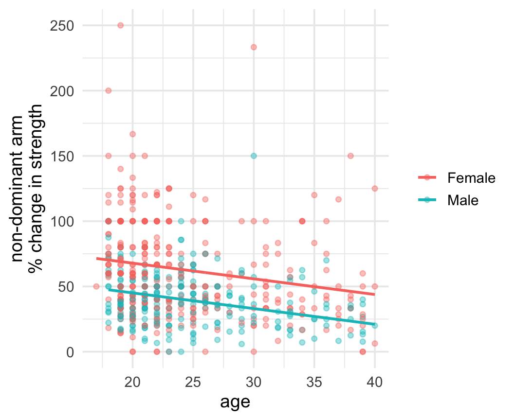
(Intercept) age sexMale
91.86 -1.20 -22.80
Each line represents the relationship between age and strength gain after adjusting for sex.
What if we have two grouping variables — and they might interact?
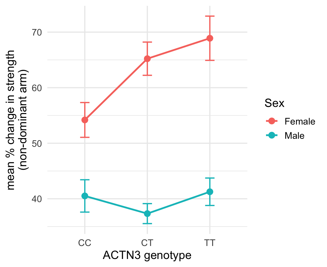
Df Sum Sq Mean Sq F value Pr(>F)
genotype 2 7043 3522 3.713 0.0250 *
sex 1 80847 80847 85.246 <2e-16 ***
genotype:sex 2 5837 2918 3.077 0.0468 *
Residuals 589 558609 948
---
Signif. codes: 0 '***' 0.001 '**' 0.01 '*' 0.05 '.' 0.1 ' ' 1
If you want to learn more, consider a minor. Core coursework after STAT218:
For more info: https://statistics.calpoly.edu/content/minors
STAT218