| mean | sd | n | se |
|---|---|---|---|
| 98.41 | 0.9162 | 39 | 0.1467 |
Applied Statistics for Life Sciences
| mean | sd | n | se |
|---|---|---|---|
| 98.41 | 0.9162 | 39 | 0.1467 |
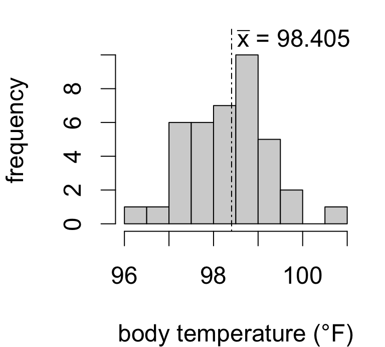
Is the true mean body temperature actually 98.6°F?
Seems plausible given our data.
But what if the sample mean were instead…
| \(\bar{x}\) | consistent with \(\mu = 98.6\)? |
|---|---|
| 98.30 | probably still yes |
| 98.15 | maybe |
| 98.00 | hesitating |
| 97.85 | skeptical |
| 97.40 | unlikely |
If the population mean is in fact 98.6°F then \[T = \frac{\bar{x} - 98.6}{s_x/\sqrt{n}} \qquad\left(\frac{\text{estimation error}}{\text{standard error}}\right)\] has a sampling distribution that is well-approximated by a \(t_{39 - 1}\) model.
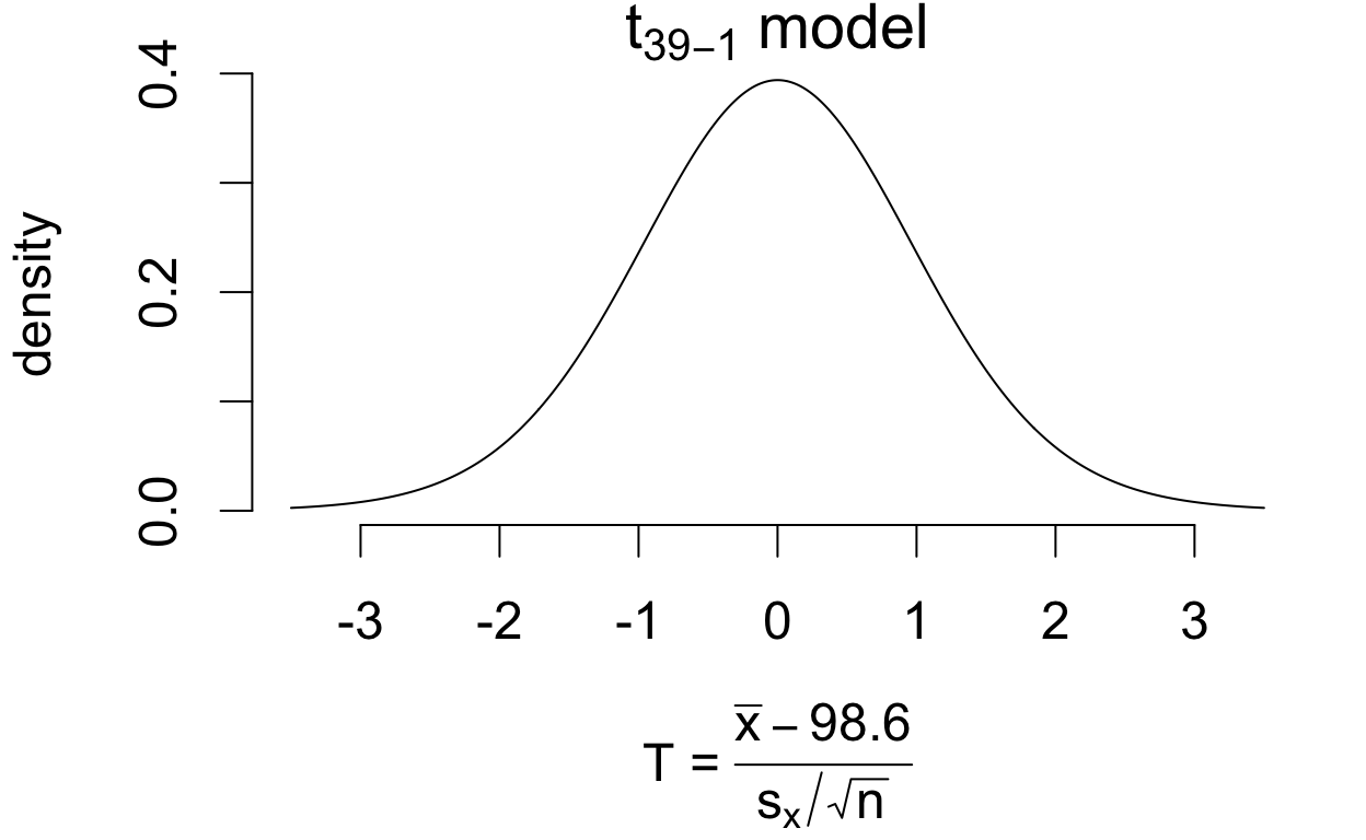
If the population mean is in fact 98.6°F then \[T = \frac{\bar{x} - 98.6}{s_x/\sqrt{n}}\qquad\left(\frac{\text{estimation error}}{\text{standard error}}\right)\] has a sampling distribution that is well-approximated by a \(t_{39 - 1}\) model.
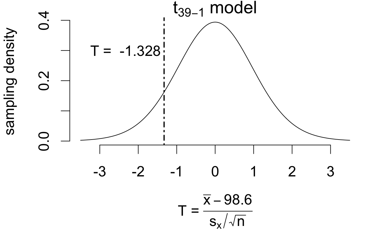
If the population mean is in fact 98.6°F then \[ T = \frac{\bar{x} - 98.6}{s_x/\sqrt{n}} \qquad\left(\frac{\text{estimation error}}{\text{standard error}}\right) \] has a sampling distribution that is well-approximated by a \(t_{39 - 1}\) model.
If the population mean is in fact 98.6°F then \[ T = \frac{\bar{x} - 98.6}{s_x/\sqrt{n}} \qquad\left(\frac{\text{estimation error}}{\text{standard error}}\right) \] has a sampling distribution that is well-approximated by a \(t_{39 - 1}\) model.

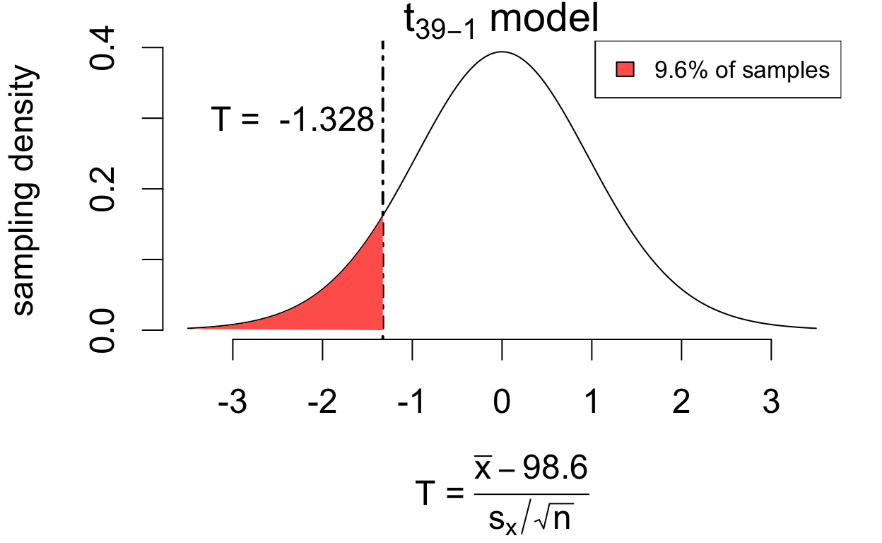
If the population mean is in fact 98.6°F then \[ T = \frac{\bar{x} - 98.6}{s_x/\sqrt{n}} \qquad\left(\frac{\text{estimation error}}{\text{standard error}}\right) \] has a sampling distribution that is well-approximated by a \(t_{39 - 1}\) model.
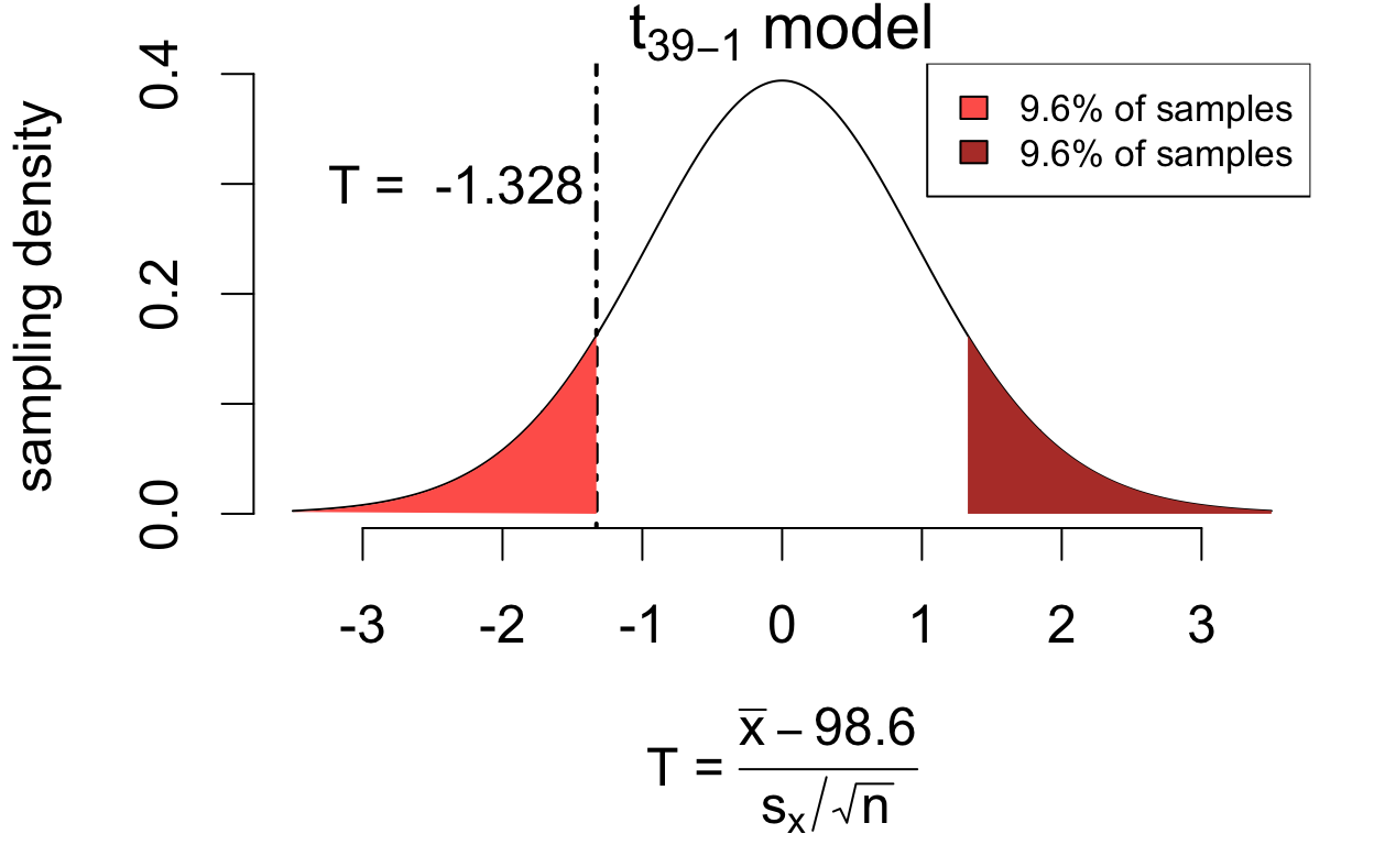
\[P(|T| > 1.328) = 0.192\]
If the hypothesis were true, we’d see at least as much estimation error 19.2% of the time. So the data are consistent with the hypothesis \(\mu = 98.6\).
If the population mean is in fact 98.6°F then \[ T = \frac{\bar{x} - 98.6}{s_x/\sqrt{n}} \qquad\left(\frac{\text{estimation error}}{\text{standard error}}\right) \] has a sampling distribution that is well-approximated by a \(t_{39 - 1}\) model.
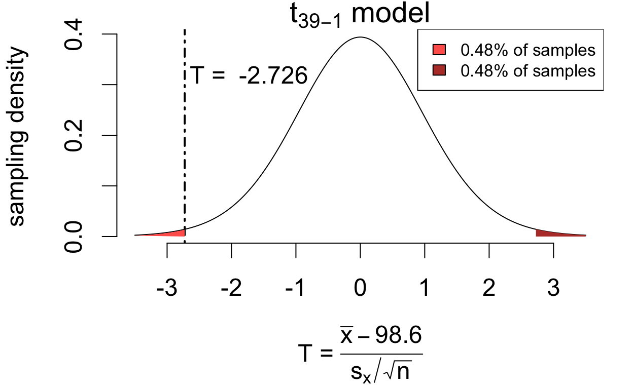
\[P(|T| > 2.726) = 0.0096\]
If the hypothesis were true, we’d see at least as much estimation error only 0.96% of the time. So the data are not consistent with the hypothesis \(\mu = 98.6\)
Tests and intervals are based on the same underlying methods.

the test tells you U.S. adults don’t sleep 8 hours:
The data provide evidence that the average U.S. adult does not sleep 8 hours per night (T = -42.53 on 3178 degrees of freedom, p < 0.0001).
the interval tells you how much they do sleep:
With 95% confidence, the mean nightly hours of sleep among U.S. adults is estimated to be between 6.91 and 7.01 hours.
… and in fact they are equivalent procedures.
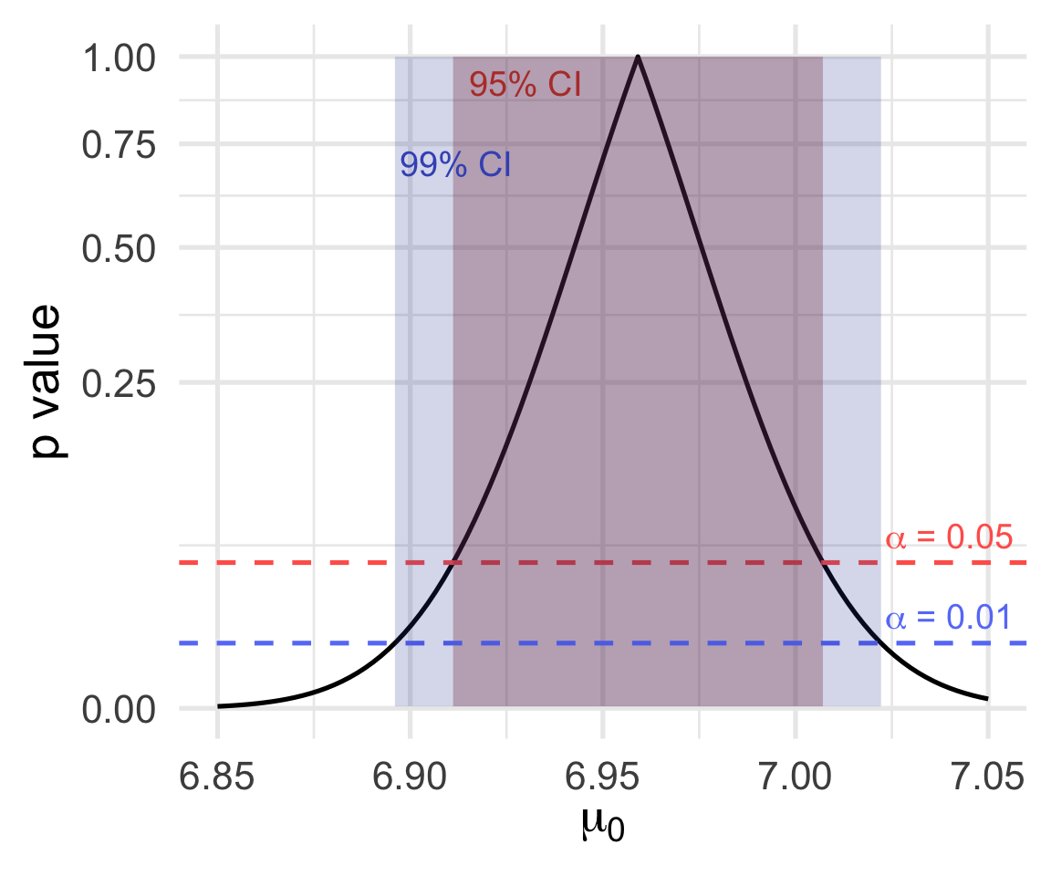
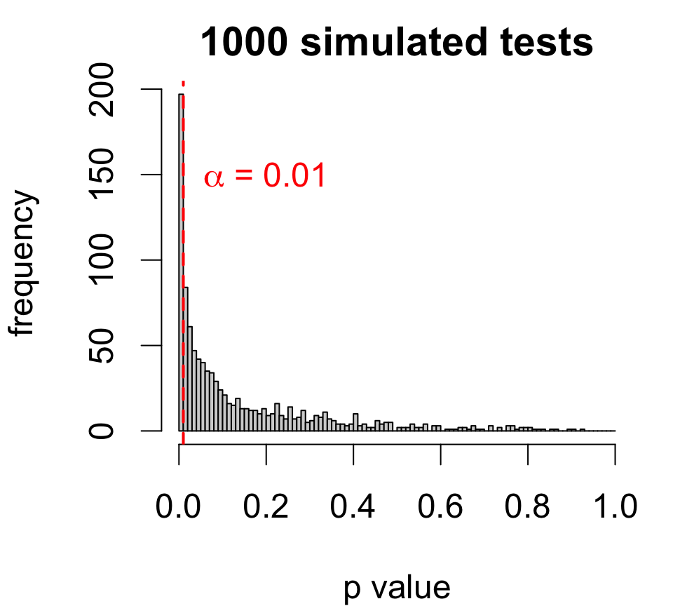
Left, \(p\)-values for a sequence of tests:
In other words:
\[\text{level $\alpha$ test rejects} \Longleftrightarrow \text{$1 - \alpha$ CI excludes}\]
Does the average U.S. adult sleep less than 7 hours?
This example leads to a lower-sided alternative:
\[ \begin{cases} H_0: &\mu = 7 \\ H_A: &\mu < 7 \end{cases} \]
The test statistic is the same as before:
\[ T = \frac{\bar{x} - 7}{SE(\bar{x})} = -1.671 \]
The lower-sided \(p\)-value is 0.0474:
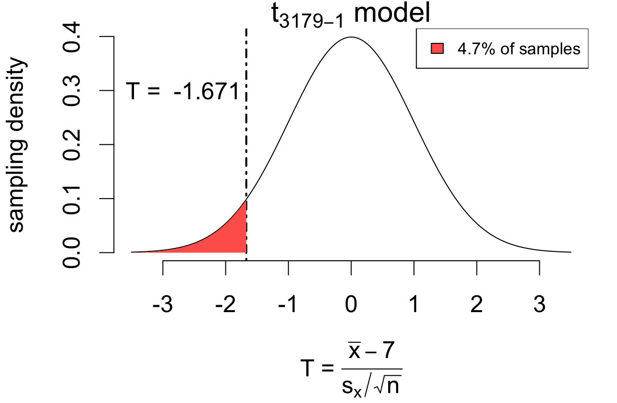
For the \(p\)-value, we look at how often \(T\) is larger in the direction of the alternative.
Does the average U.S. adult sleep more than 7 hours?*
Now the alternative is in the opposite direction:
\[ \begin{cases} H_0: &\mu = 7 \\ H_A: &\mu > 7 \end{cases} \]
The test statistic is the same as before:
\[ T = \frac{\bar{x} - 7}{SE(\bar{x})} = -1.671 \]
The upper-sided \(p\)-value is 0.9526:

For the \(p\)-value, we look at how often \(T\) is larger in the direction of the alternative.
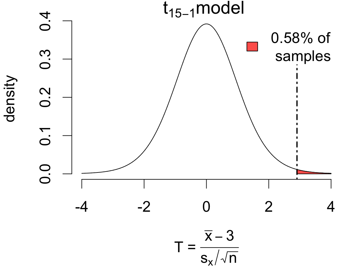
If in fact \(\mu = 3\), then according to the \(t\) model 0.58% of samples would produce an error of this magnitude or more in the direction of the alternative:
    One Sample t-test

data:  ddt
t = 2.9059, df = 14, p-value = 0.005753
alternative hypothesis: true mean is greater than 3
95 percent confidence interval:
 3.129197      Inf
sample estimates:
mean of x
    3.328
The data provide strong evidence that mean DDT in kale exceeds 3ppm (T = 2.9059 on 14 degrees of freedom, p = 0.0058). With 95% confidence, the mean DDT is estimated to be at least 3.129, with a point estimate of 3.32 (SE: 0.1129).
Notice the one-sided interval! (Inf = \(\infty\).) This is called a “lower confidence bound”.
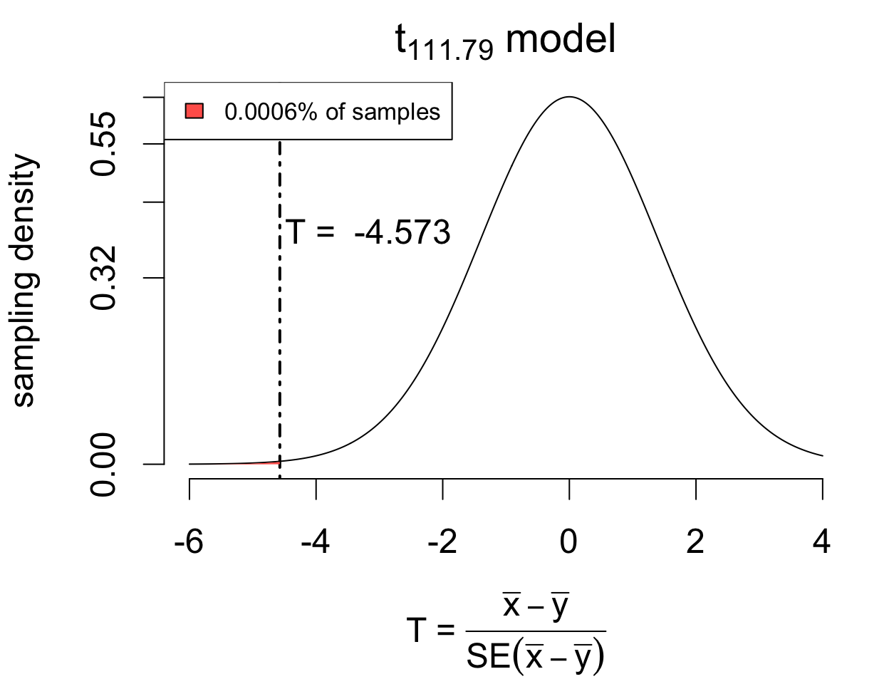
If \(x_1, \dots, x_{58}\) are the 1976 observations and \(y_1, \dots, y_{65}\) are the 1978 observations:
Inference uses a new \(T\) statistic:
\[ T = \frac{(\bar{x} - \bar{y}) - \delta_0}{SE(\bar{x} - \bar{y})} \]

The two-sample test is appropriate whenever two one-sample tests would be.
In other words, the test assumes that both samples are either:
To check, simply inspect each histogram.
The two-sample test is appropriate whenever two one-sample tests would be.
In other words, the test assumes that both samples are either:
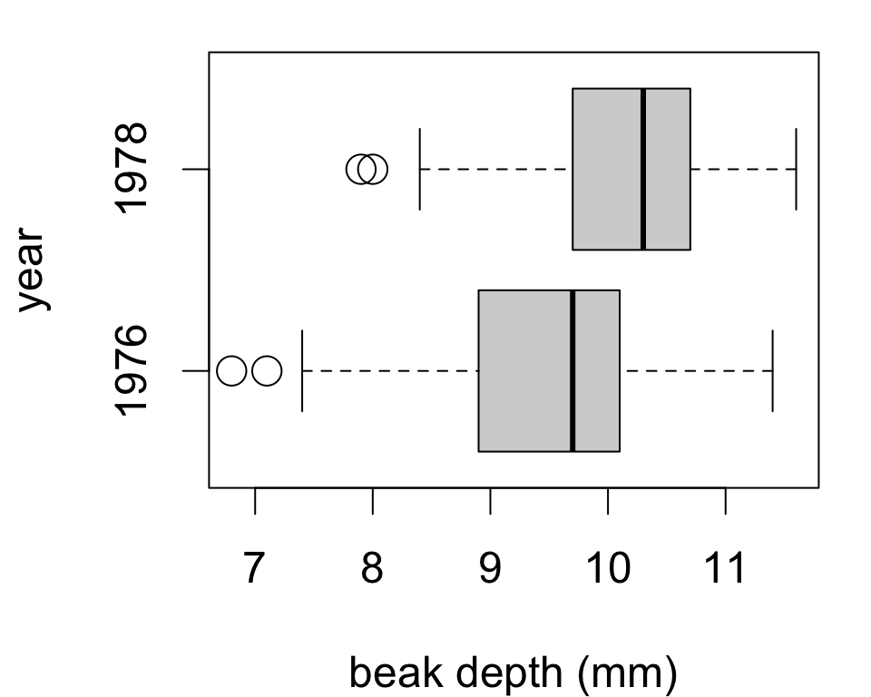
Could also check side-by-side boxplots for:
This is also a nice visualization of differences between samples.
Summary stats for cloud data:
| treatment | mean | sd | n |
|---|---|---|---|
| seeded | 442 | 650.8 | 26 |
| unseeded | 164.6 | 278.4 | 26 |
We can approximate the type II error rate by:
If in fact the effect size is exactly 277, a level 1% test with similar data will fail to reject 80.3% of the time!
Summary stats for cloud data:
| treatment | mean | sd | n |
|---|---|---|---|
| seeded | 442 | 650.8 | 26 |
| unseeded | 164.6 | 278.4 | 26 |
Type II error rate depends on effect size:
If in fact the effect size is exactly 400, a level 1% test with similar data will fail to reject 57.9% of the time.
Summary stats for cloud data:
| treatment | mean | sd | n |
|---|---|---|---|
| seeded | 442 | 650.8 | 26 |
| unseeded | 164.6 | 278.4 | 26 |
Type II error rate depends on effect size:
If in fact the effect size is exactly 100, a level 1% test with similar data will fail to reject 96.3% of the time.
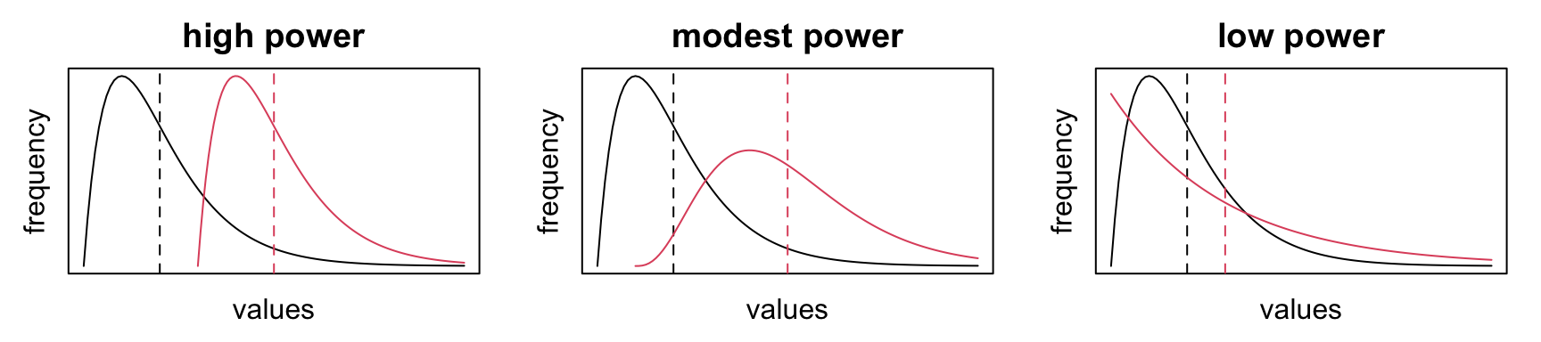
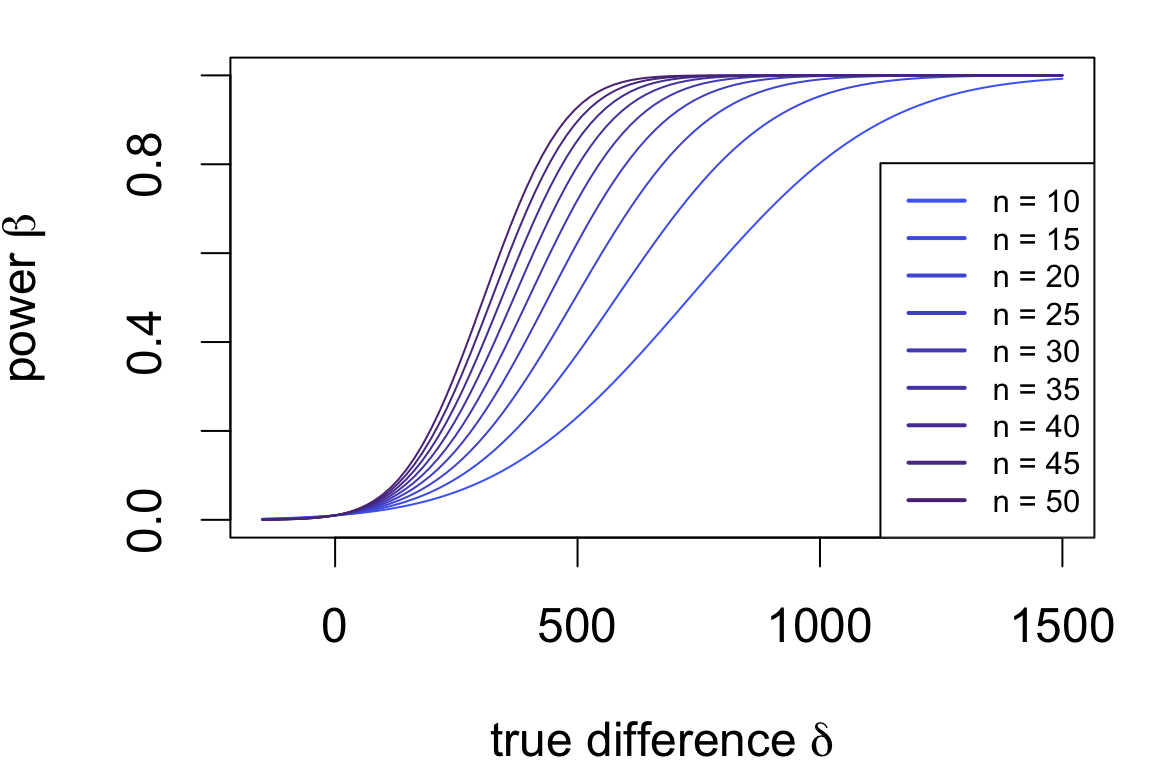
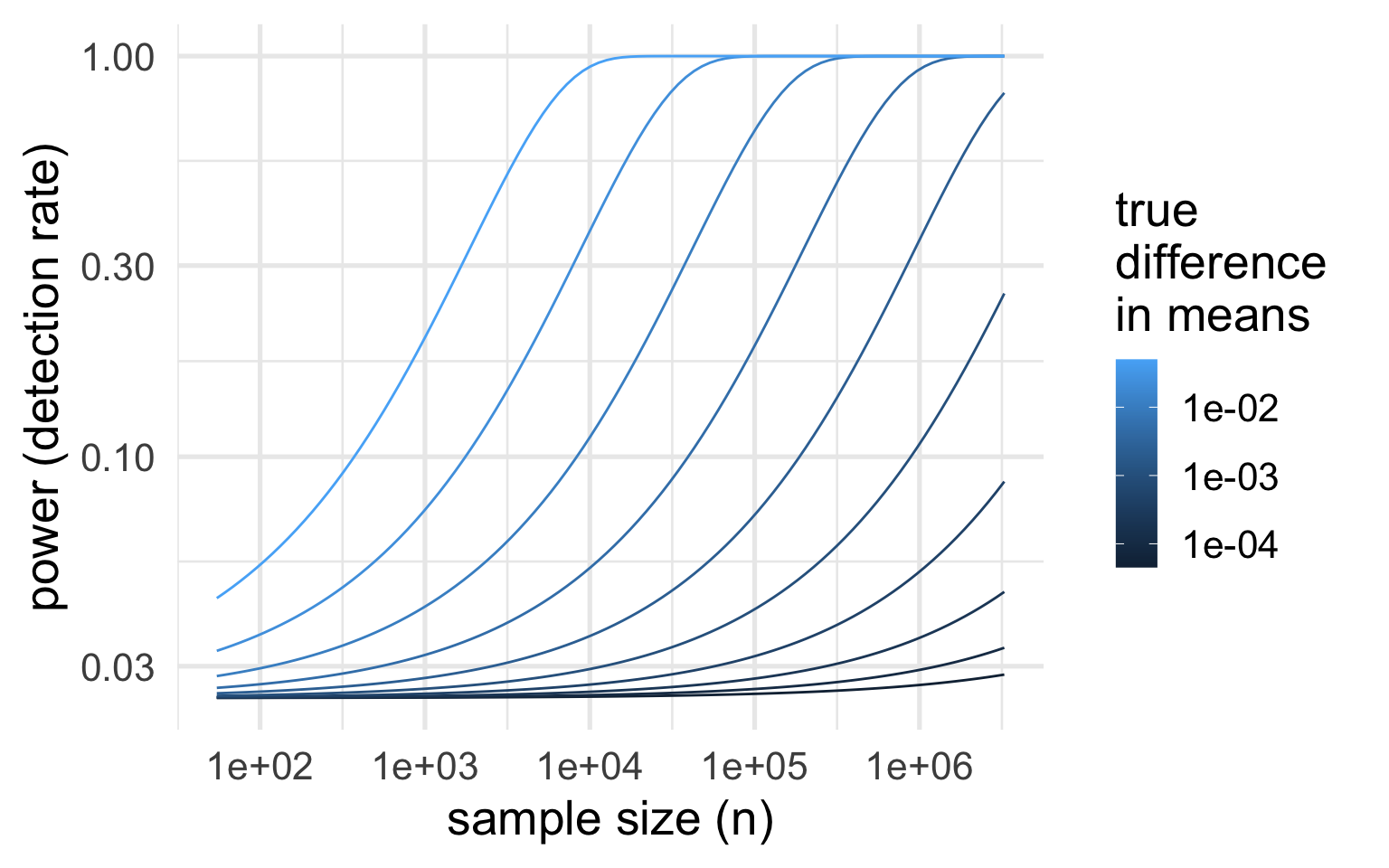
Power is usually represented as a curve depending on the true difference.
Power curves for the test applied to the cloud data:

Assumptions:
Which sample size achieves a specific \(\beta, \delta\)?
Does mean body temperature differ between men and women?
Test \(H_0: \mu_F = \mu_M\) against \(H_A: \mu_F \neq \mu_M\)
    Welch Two Sample t-test

data:  body.temp by sex
t = 1.7118, df = 34.329, p-value = 0.09595
alternative hypothesis: true difference in means between group female and group male is not equal to 0
95 percent confidence interval:
 -0.09204497  1.07783444
sample estimates:
mean in group female   mean in group male
            98.65789             98.16500
Suggestive but insufficient evidence that mean body temperature differs by sex.
Notice: estimated difference (F - M) is 0.493 °F (SE 0.2879)
If you collect enough data, you can detect an arbitrarily small difference in means.
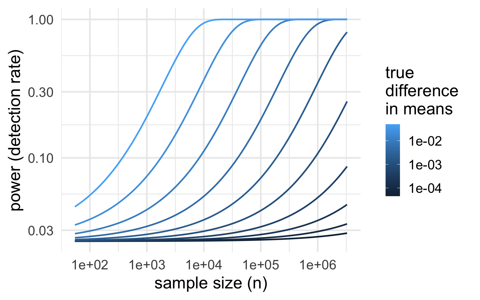
So keep in mind:
It’s a good idea to always check your point estimates and ask whether findings are practically meaningful.
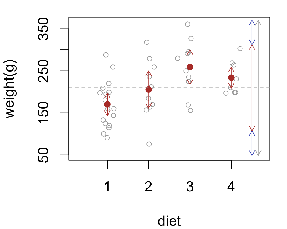
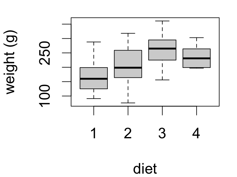
Chick weights at 20 days of age by diet:

Here we have four means to compare.
| diet | mean | se | sd | n |
|---|---|---|---|---|
| 1 | 170.4 | 13.45 | 55.44 | 17 |
| 2 | 205.6 | 22.22 | 70.25 | 10 |
| 3 | 258.9 | 20.63 | 65.24 | 10 |
| 4 | 233.9 | 12.52 | 37.57 | 9 |
This is experimental data: chicks were randomly allocated one of the four diets.
Here are two made-up examples of the same four sample means with different SEs.
Why does it look like there’s a difference at right but not at left?
Think about the \(t\)-test: we say there’s a difference if \(T = \frac{\text{estimate} - \text{hypothesis}}{\text{variability}}\) is large.
Same idea here: we see differences if they are big relative to the variability in estimates.
Partitioning variation into two or more components is called “analysis of variance”
For the chick data, two sources of variability:
group variability between diets
error variability among chicks
The analysis of variance (ANOVA) model:
\[\color{grey}{\text{total variation}} = \color{red}{\text{group variation}} + \color{blue}{\text{error variation}}\]
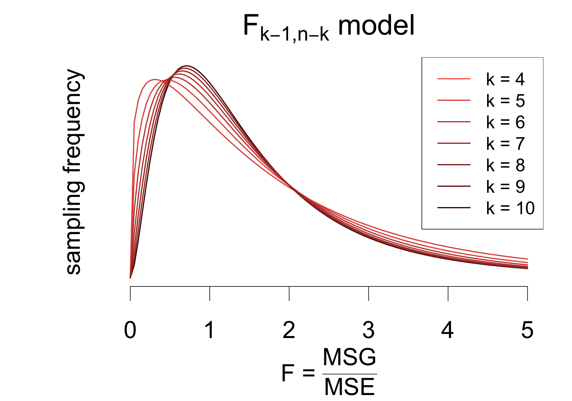
We’ll base the test on the ratio \(F = \frac{\color{red}{\text{group variation}}}{\color{blue}{\text{error variation}}}\) and reject \(H_0\) if the ratio is large enough.
Provided that
the \(F\) statistic has a sampling distribution well-approximated by an \(F_{k - 1, n - k}\) model.
To test the hypotheses:
\[ \begin{cases} H_0: &\mu_1 = \mu_2 = \mu_3 = \mu_4 \\ H_A: &\mu_i \neq \mu_j \quad\text{for some}\quad i \neq j \end{cases} \] Calculate the \(F\) statistic:
# ingredients of mean squares
k <- nrow(chicks.summary)
n <- nrow(chicks)
n.i <- chicks.summary$n
xbar.i <- chicks.summary$mean
s.i <- chicks.summary$sd
xbar <- mean(chicks$weight)

# mean squares
msg <- sum(n.i*(xbar.i - xbar)^2)/(k - 1)
mse <- sum((n.i - 1)*s.i^2)/(n - k)

# f statistic
fstat <- msg/mse
fstat
[1] 5.463598And reject \(H_0\) when \(F\) is large.
\[ \begin{cases} H_0: &\mu_1 = \mu_2 = \mu_3 = \mu_4 \\ H_A: &\mu_i \neq \mu_j \quad\text{for some}\quad i \neq j \end{cases} \]
\(F = \frac{\color{red}{\text{group variation}}}{\color{blue}{\text{error variation}}} = \frac{MSG}{MSE} = 5.4636\).
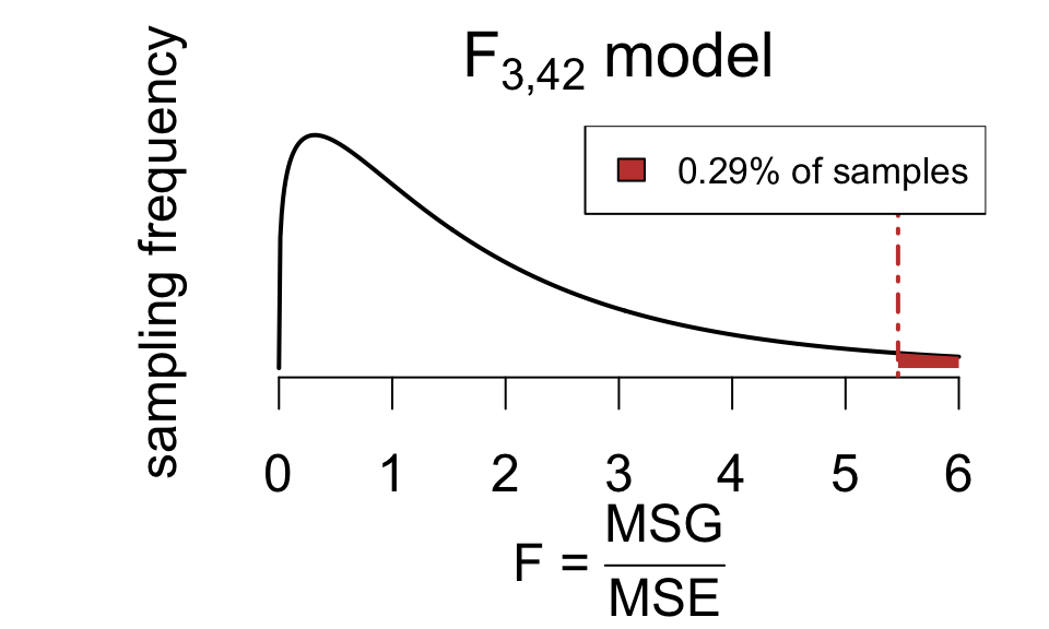
F = 5.4636 means the variation in weight attributable to diets is 5.46 times greater than individual variation among chicks.
The \(p\)-value for the test is 0.0029:
if there is truly no difference in means, then under 1% of samples (about 2 in 1000) would produce at least as much diet-to-diet variability as we observed
so in this case we reject \(H_0\) at the 1% level
From data on lifespans of lab mice fed calorie-restricted diets:
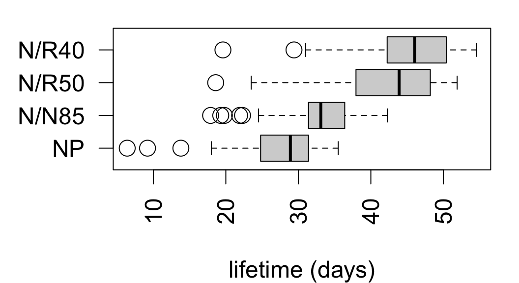
| diet | mean | sd | n |
|---|---|---|---|
| NP | 27.4 | 6.134 | 49 |
| N/N85 | 32.69 | 5.125 | 57 |
| N/R50 | 42.3 | 7.768 | 71 |
| N/R40 | 45.12 | 6.703 | 60 |
ANOVA omnibus test:
\[ \begin{align*} &H_0: \mu_\text{NP} = \mu_\text{N/N85} = \mu_\text{N/R50} = \mu_\text{N/R40} \\ &H_A: \text{at least two means differ} \end{align*} \]
             Df Sum Sq Mean Sq F value Pr(>F)
diet          3  11426    3809   87.41 <2e-16 ***
Residuals   233  10152      44
---
Signif. codes:  0 '***' 0.001 '**' 0.01 '*' 0.05 '.' 0.1 ' ' 1
The data provide evidence that diet restriction has an effect on mean lifetime among mice (F = 87.41 on 3 and 233 degrees of freedom, p < 0.0001).
From data on weight change among 72 young anorexic women after a period of therapy:
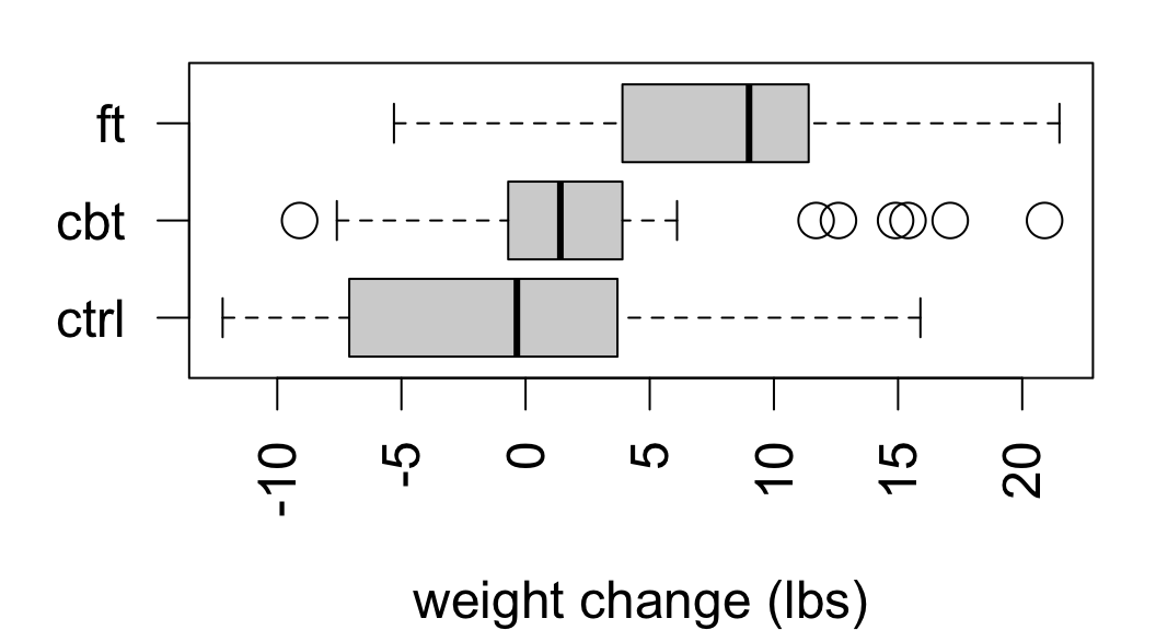
| treat | post - pre | sd | n |
|---|---|---|---|
| ctrl | -0.45 | 7.989 | 26 |
| cbt | 3.007 | 7.309 | 29 |
| ft | 7.265 | 7.157 | 17 |
ANOVA omnibus test: \[ \begin{align*} &H_0: \mu_\text{ctrl} = \mu_\text{cbt} = \mu_\text{ft} \\ &H_A: \text{at least two means differ} \end{align*} \]
            Df Sum Sq Mean Sq F value Pr(>F)
treat        2    615  307.32   5.422 0.0065 **
Residuals   69   3911   56.68
---
Signif. codes:  0 '***' 0.001 '**' 0.01 '*' 0.05 '.' 0.1 ' ' 1
The data provide evidence of an effect of therapy on mean weight change among young women with anorexia (F = 5.422 on 2 and 69 degrees of freedom, p = 0.0065).
\[ \begin{align*} &H_0: \mu_\text{NP} = \mu_\text{N/N85} = \mu_\text{N/R50} = \mu_\text{N/R40} \\ &H_A: \text{at least two means differ} \end{align*} \]

             Df Sum Sq Mean Sq F value Pr(>F)
diet          3  11426    3809   87.41 <2e-16 ***
Residuals   233  10152      44
---
Signif. codes: 0 '***' 0.001 '**' 0.01 '*' 0.05 '.' 0.1 ' ' 1# Effect Size for ANOVA (Type I)
Parameter | Eta2 | 95% CI
-------------------------------
diet | 0.53 | [0.44, 0.60]The ANOVA tells us there’s evidence that caloric intake affects mean lifespan.
So which means differ and by how much?
For multiple intervals we can distinguish two types of coverage.
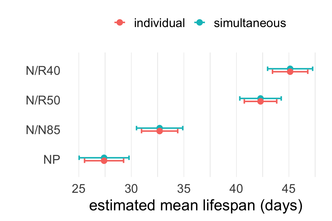
The Bonferroni correction for \(k\) intervals consists in changing the individual coverage level to \(\left(1 - \frac{\alpha}{k}\right)\%\).
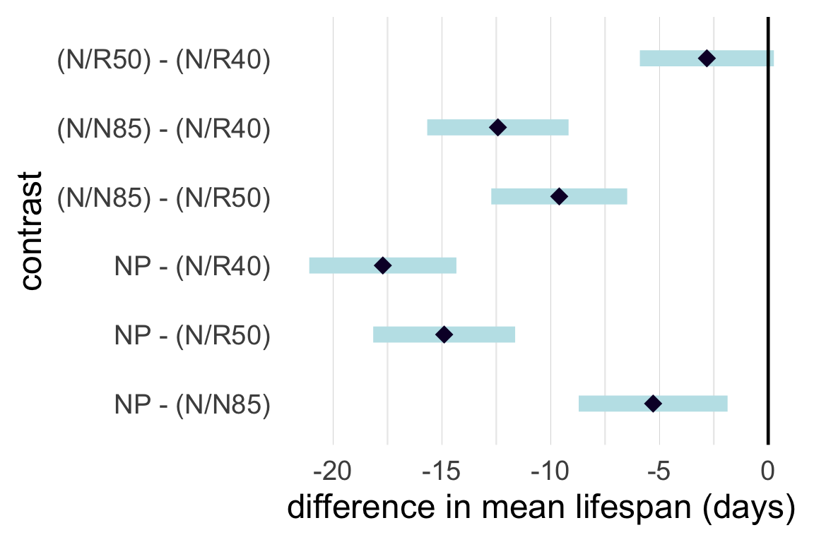
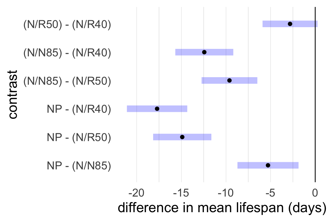
Another option is to visualize the pairwise comparison inferences by displaying simultaneous 95% intervals.
Easy to spot significant contrasts:
We can use the log-contrasts to estimate a response curve relating caloric reduction and change in median lifespan.
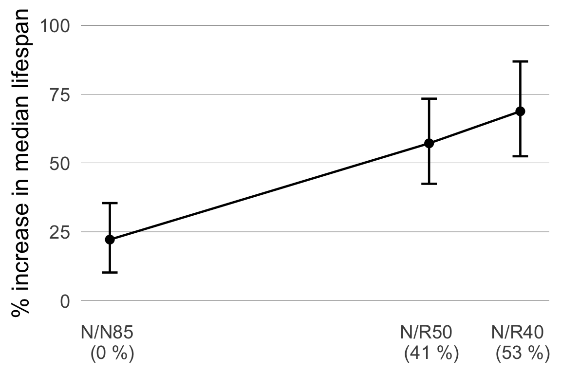
Simplifying heuristics:
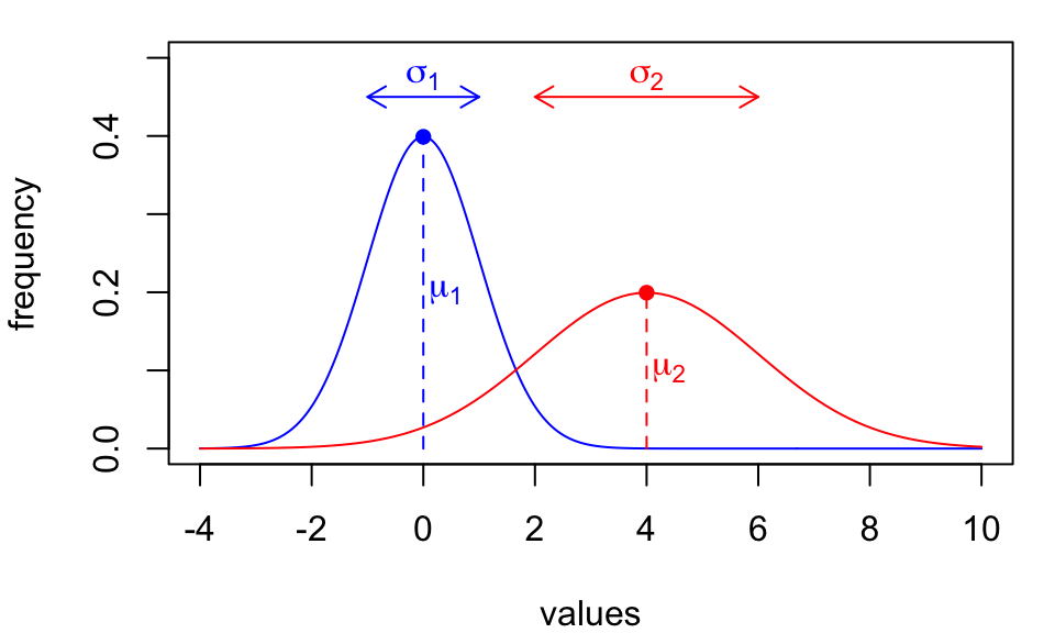
The inferences we’ve developed so far are based on simple statistical models:
Both models assume underlying data distributions are described by…
We call these called parametric methods.
Parametric model assumptions don’t always hold.
DDT concentrations (ppm) in kale samples.
With only \(n = 12\) observations, it’s hard to assess the shape of the distribution.
Serum cholesterol (mg/L) on two diets.
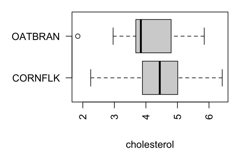
The distribution for the oat bran group is right-skewed with an outlier to the left.
Here assumptions may not hold:
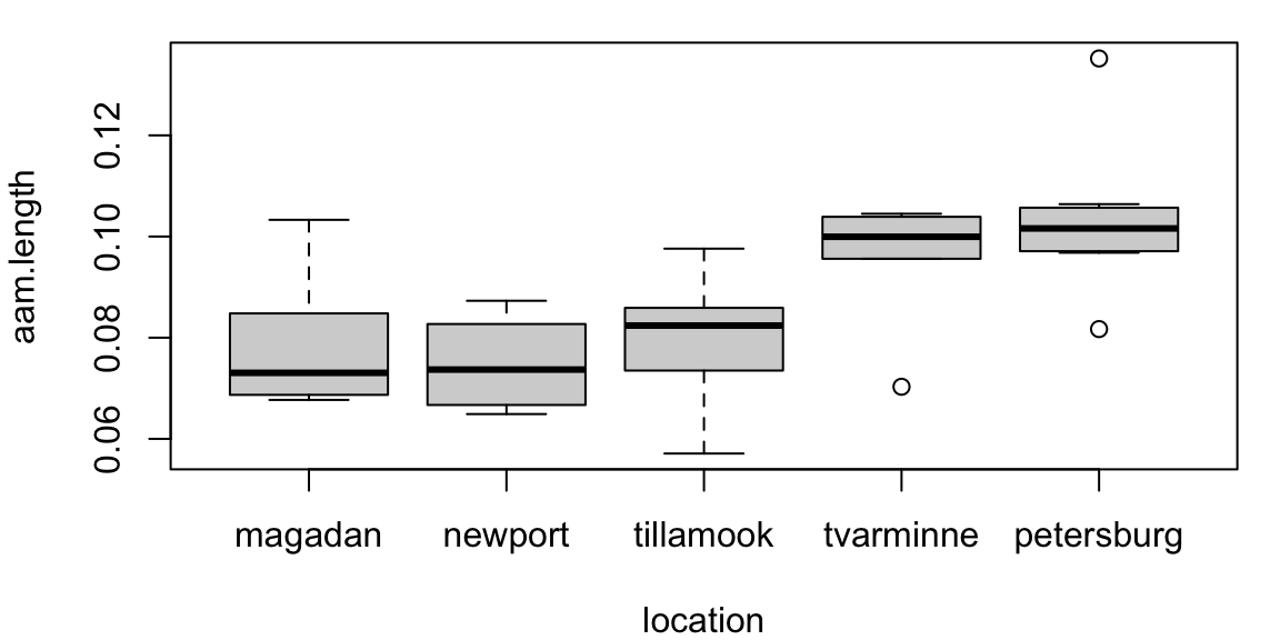
\[ \begin{cases} H_0: &c_M = c_N = c_{Ti} = c_{Tv} = c_P \\ H_A: &c_i \neq c_j \quad\text{ for some }\quad i\neq j \end{cases} \]
An ANOVA-like test can be formulated using ranks of pooled observations:
\[ U = \frac{\sum_{j = 1}^k n_j (\bar{r}_j - \bar{r})^2}{\sum_{i = 1}^n (r_i - \bar{r})^2} \qquad \left(\frac{\text{group variation}}{\text{total variation}}\right) \]
If there are location differences, \(U\) will be large.
The omnibus test in ANOVA gives a similar result:
            Df   Sum Sq   Mean Sq F value   Pr(>F)
location     4 0.004520 0.0011299   7.121 0.000281 ***
Residuals   34 0.005395 0.0001587
---
Signif. codes:  0 '***' 0.001 '**' 0.01 '*' 0.05 '.' 0.1 ' ' 1
But the pairwise comparisons differ:
# A tibble: 4 × 6
  contrast               estimate      SE    df t.ratio p.value
  <chr>                     <dbl>   <dbl> <dbl>   <dbl>   <dbl>
1 magadan - petersburg    -0.0254 0.00652    34   -3.90 0.00430
2 newport - tvarminne     -0.0209 0.00680    34   -3.07 0.0417
3 newport - petersburg    -0.0286 0.00652    34   -4.39 0.00103
4 tillamook - petersburg  -0.0232 0.00621    34   -3.74 0.00670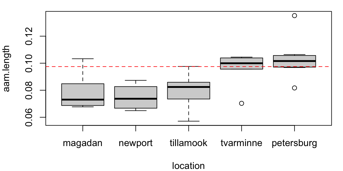
The parametric test is more sensitive to skewness and outliers!
Two-sample and ANOVA-type rank-based inference procedures detect location shifts only.
While we write the hypotheses in terms of centers by convention, really we’re testing:
These tests are not sensitive to alternatives in which centers differ due to shape.