A study is an effort to collect data in order to answer one or more research questions.
studies must be well-matched to research questions to provide good answers
how data are obtained is just as important as how the resulting data are analyzed
no analysis, no matter how sophisticated will rescue a poorly conceived study
A study unit is the smallest object or entity that is measured in a study; also called experimental unit or observational unit.
Sampling
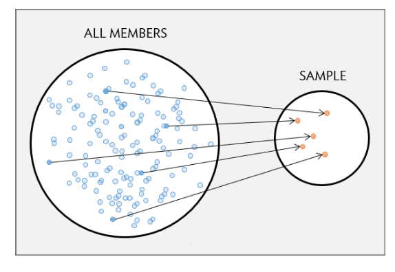
Study units should be chosen so as to represent a larger collection or “population”.
A study population is a collection of all study units of interest.
A sample is a subcollection:
probability sample: all study units have some known “inclusion probability” or chance of being selected
nonrandom/convenience sample: inclusion probabilities are not known
The gold standard is the simple random sample: all inclusion probabilities are equal.
ensures samples of a fixed size from the population are exchangeable and thus “representative”
justifies inferences about the population based on the sample
Two types of studies
Observational studies collect data from an existing situation without intervention.
Aim is to detect associations and patterns
Can’t be used to infer causal relationships owing to possible unmeasured confounding
Experiments collect data from a situation in which one or more interventions have been introduced by the investigator.
Interventions are (supposed to be) randomized among study units
Aim is to draw conclusions about the causal effect of interventions
Stronger form of scientific evidence than an observational study
LEAP Study
Learning early about peanut allergy (LEAP) study:
640 infants in UK with eczema or egg allergy but no peanut allergy enrolled
each infant randomly assigned to peanut consumption and peanut avoidance groups
peanut consumption: fed 6g peanut protein daily until 5 years old
peanut avoidance: no peanut consumption until 5 years old
at 5 years old, oral food challenge (OFC) allergy test administered
13.3% of the avoidance group developed allergies, compared with 1.9% of the consumption group
Study characteristics
Study type: experiment
Study population: UK infants with eczema or egg allergy but no peanut allergy
Sample: 640 infants from population
Treatments: peanut consumption; peanut avoidance
Treatment allocation: completely randomized
Study outcome: development of peanut allergy by 5 years of age
Study results
Moderated peanut consumption causes a reduction in the likelihood of developing an allergy among infants with prior risk (eczema or egg allergies).
Why randomize?
Randomization eliminates confounding by ensuring that study interventions are independent of all extraneous conditions.
no association is possible between study intervention and unobserved variables
if outcomes differ systematically according to the intervention, you can be certain that the intervention is responsible
flowchart TD
  A(unobserved variables) x-.-x B(study conditions)
  A --- C(outcome)
For example, imagine an observational version of the LEAP study in which allergy rates are compared between children who consumed peanuts as infants and those who didn’t.
those with reactions are more likely to become avoiders
could inflate the observed difference relative to the true effect
Randomizing consumption regimens eliminates this possibility.
Data semantics
Data are a set of measurements.
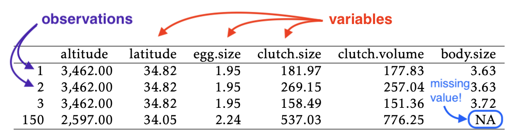
A variable is any measured attribute of study units.
An observation is a measurement of one or more variables taken on one particular study unit.
It is usually expedient to arrange data values in a table in which each row is an observation and each column is a variable:
LEAP example
A table showing the observations and variables for the LEAP study would look like this:
participant.ID
treatment.group
ofc.test.result
LEAP_100522
Peanut Consumption
PASS OFC
LEAP_103358
Peanut Consumption
PASS OFC
LEAP_105069
Peanut Avoidance
PASS OFC
LEAP_105328
Peanut Consumption
PASS OFC
The table you saw in the reading was a summary of the data (not the data itself):
FAIL OFC
PASS OFC
Peanut Avoidance
36
227
Peanut Consumption
5
262
Numeric and categorical variables
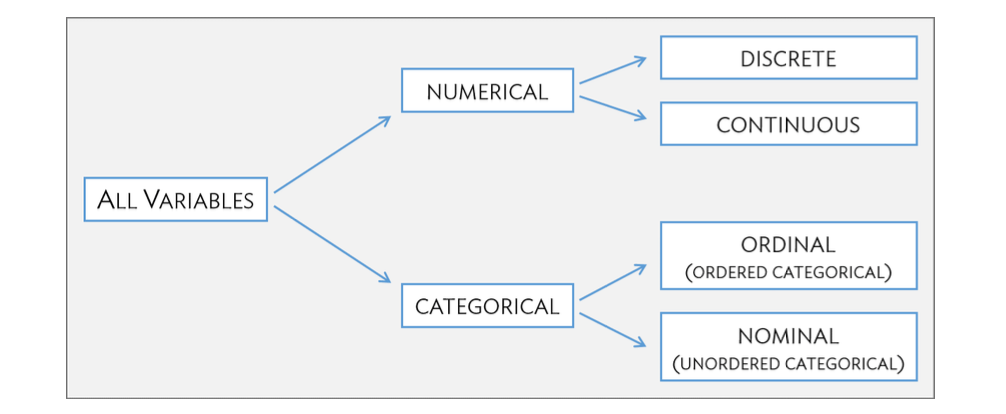
Variables are classified according to their values. Values can be one of two different types:
A variable is numeric if its value is a number
A variable is categorical if its value is a category, usually recorded as a name or label
For example:
the value of sex can be male or female, so it is categorical
whereas age (in years) can be any positive integer, so it is numeric
Variable subtypes
Further distinctions are made based on the type of number or type of category used to measure an attribute. Can you match the subtypes to the variables at right?
age
hispanic
grade
weight
15
not
10
78.02
18
hispanic
12
78.47
17
not
11
95.26
18
not
12
95.26
a numerical variable is discrete if there are ‘gaps’ between its possible values
a numerical variable is continuous if there are no such gaps
a categorical variable is nominal if its levels are not ordered
a categorical variable is ordinal if its levels are ordered
Many ways to measure attributes
Variable type (or subtype) is not an inherent quality — attributes can often be measured in many different ways.
For instance, age might be measured as either a discrete, continuous, or ordinal variable, depending on the situation:
Age (years)
Age (minutes)
Age (brackets)
12
6307518.45
10-18
8
4209187.18
5-10
21
11258103.08
18-30
Numeric variables can always be discretized into categorical variables.
Your turn
Classify each variable as nominal, ordinal, discrete, or continuous:
ndrm.ch
genotype
sex
age
race
bmi
33.3
CT
Female
19
Caucasian
21.01
71.4
CT
Female
18
Other
23.18
37.5
CC
Female
21
Caucasian
28.92
50
CC
Female
28
Asian
21.16
Data are from an observational study investigating demographic, physiological, and genetic characteristics associated with muscle strength.
ndrm.ch is change in strength in nondominant arm after resistance training
genotype indicates genotype at a particular location within the ACTN3 gene
Recap
Data semantics
Data are a collection of measurements taken on a sample of study units:
measured attributes are called variables
per-unit measurements are called observations
Variables are classified by their values:
categorical data: ordinal (ordered) or nominal (unordered) categories
numeric data: continuous (no ‘gaps’) or discrete (‘gaps’) numbers
Data structures
Observations of many variables are stored as data frames:
# 3 observations of age and sexhead(subjects, 3)
  subject.id age sex
1         11  24   m
2          2  31   m
3         31  17   f
Observations of a single variable are stored as vectors:
# extract age variableages <- subjects$ageages
[1] 24 31 17
Descriptive statistics
Dataset: FAMuSS study
Observational study of 595 individuals comparing change in arm strength before and after resistance training between genotypes for a region of interest on the ACTN3 gene.
Pescatello, L. S., et al. (2013). Highlights from the functional single nucleotide polymorphisms associated with human muscle size and strength or FAMuSS study. BioMed research international.
Example data rows
ndrm.ch
drm.ch
sex
age
race
height
weight
genotype
bmi
40
40
Female
27
Caucasian
65
199
CC
33.11
25
0
Male
36
Caucasian
71.7
189
CT
25.84
40
0
Female
24
Caucasian
65
134
CT
22.3
125
0
Female
40
Caucasian
68
171
CT
26
Summary statistics
A statistic is, mathematically, a function of the values of two or more observations
For numeric variables, the most common summary statistic is the average value:
\[\text{average} = \frac{\text{sum of values}}{\text{# observations}}\]
For example, the average percent change in nondominant arm strength was 53.291%.
For categorical variables, the most common summary statistic is a proportion:
\[\text{proportion}_i = \frac{\text{# observations in category } i}{\text{# observations}}\]
For example:
Genotype proportions
CC
CT
TT
0.2908
0.4387
0.2706
Mathematical notation
Typically, a set of observations is written as:
\[x_1, x_2, \dots, x_n\]
\(x\) represents the variable (e.g., genotype, age, percent change, etc.)
\(i\) (subscript) Indexes observations: \(x_i\) is the \(i\)th observation
\(n\) is the total Number of observations
The sum of the observations is written \(\sum_i x_i\), where the symbol \(\sum\) stands for ‘summation’. This is useful for writing the formula for computing an average:
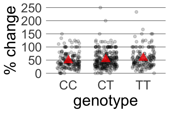
Descriptive statistics refers to analysis of sample characteristics using summary statistics (functions of data) and/or graphics.
For example:
genotype
avg.change.strength
n.obs
TT
58.08
161
CT
53.25
261
CC
48.89
173
We call these descriptions and not inferences because they describe the sample:
Among study participants, those with genotype TT (n = 161) had the greatest average change in nondominant arm strength (58.08%).
The appropriate type of data summary depends on the variable type(s)
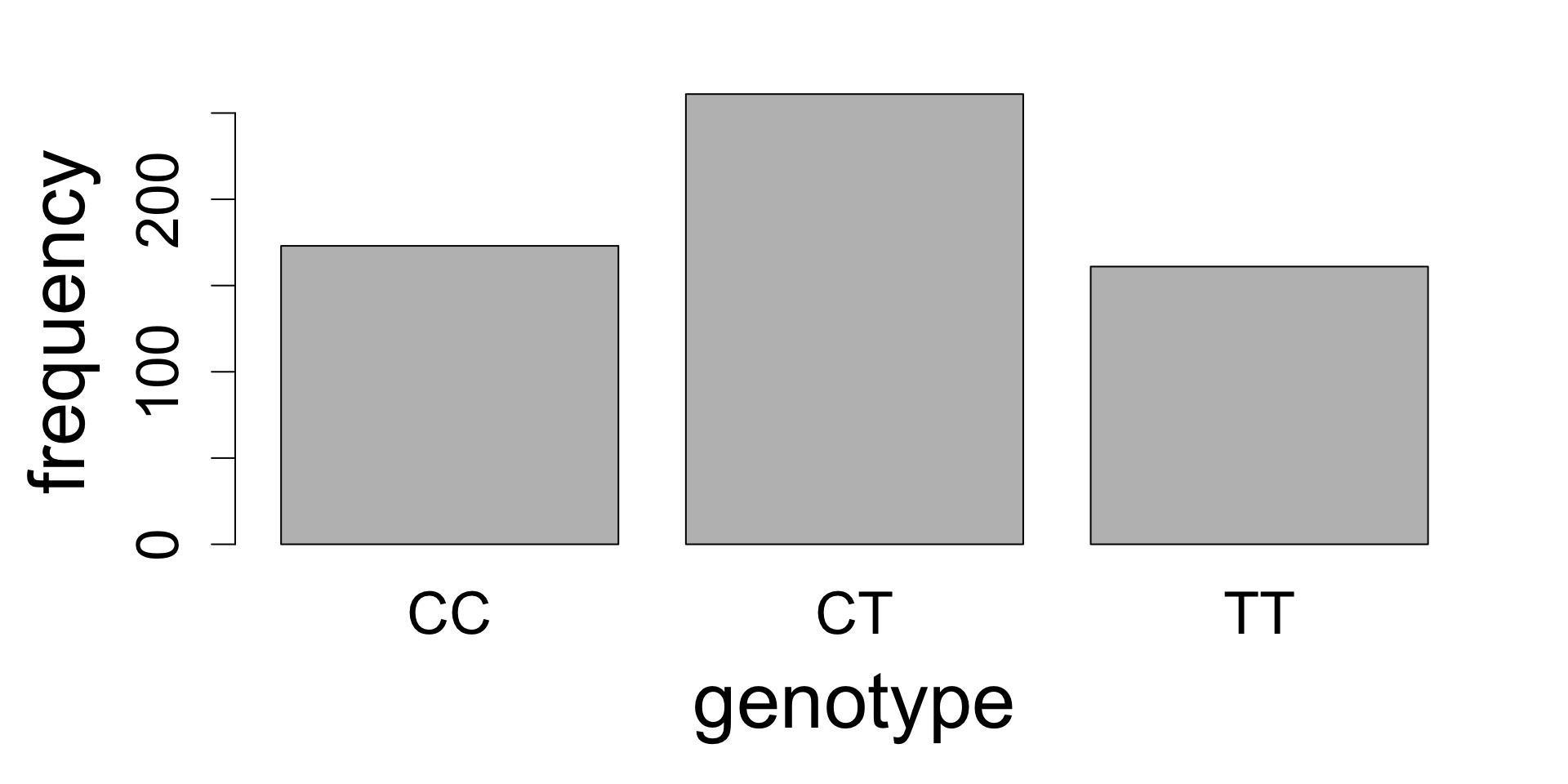
Categorical frequency distributions
For categorical variables, the frequency distribution is simply an observation count by category. For example:
Raw data
participant.id
genotype
494
TT
510
TT
216
CT
19
TT
278
CT
86
TT
Frequency distribution
CC
CT
TT
173
261
161
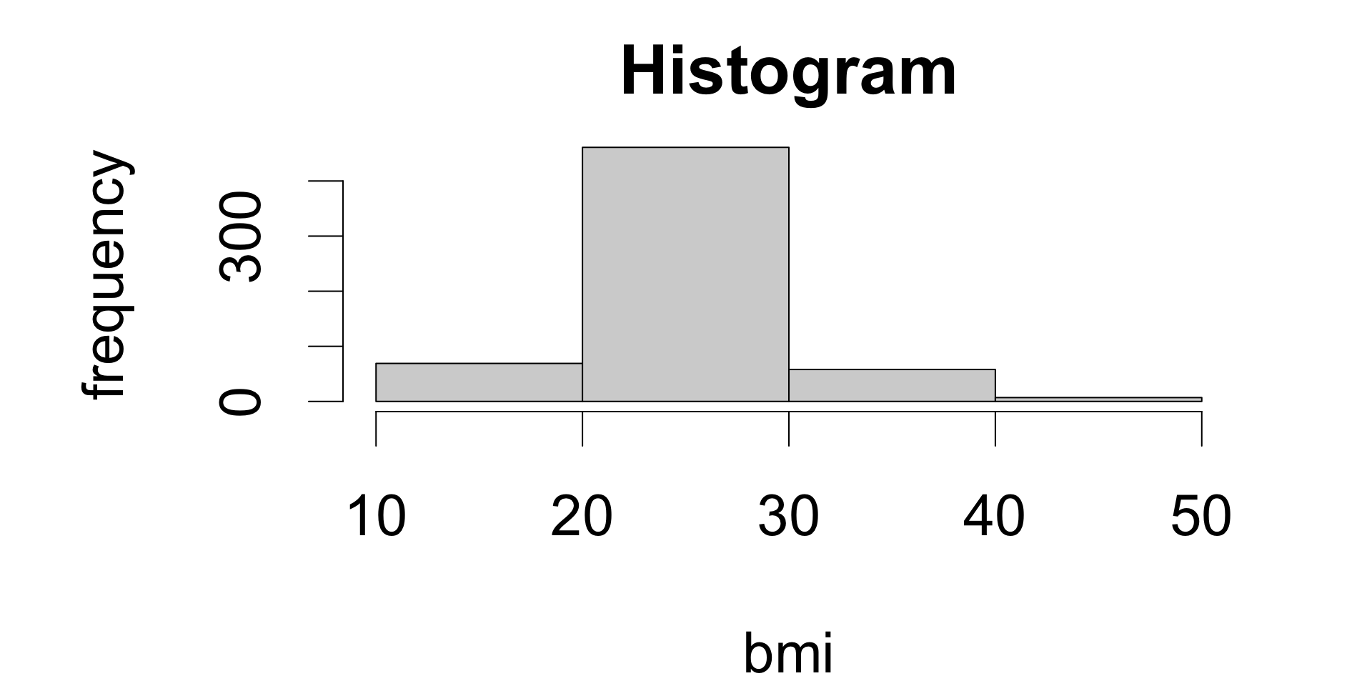
Numeric frequency distributions
Frequency distributions of numeric variables are observation counts by “bins”: small intervals of a fixed width.
A plot of a numeric frequency distribution is called a histogram.
Data table
participant.id
bmi
194
22.3
141
20.76
313
23.48
522
29.29
504
42.28
273
20.34
Frequency distribution
(10,20]
(20,30]
(30,40]
(40,50]
69
461
58
7
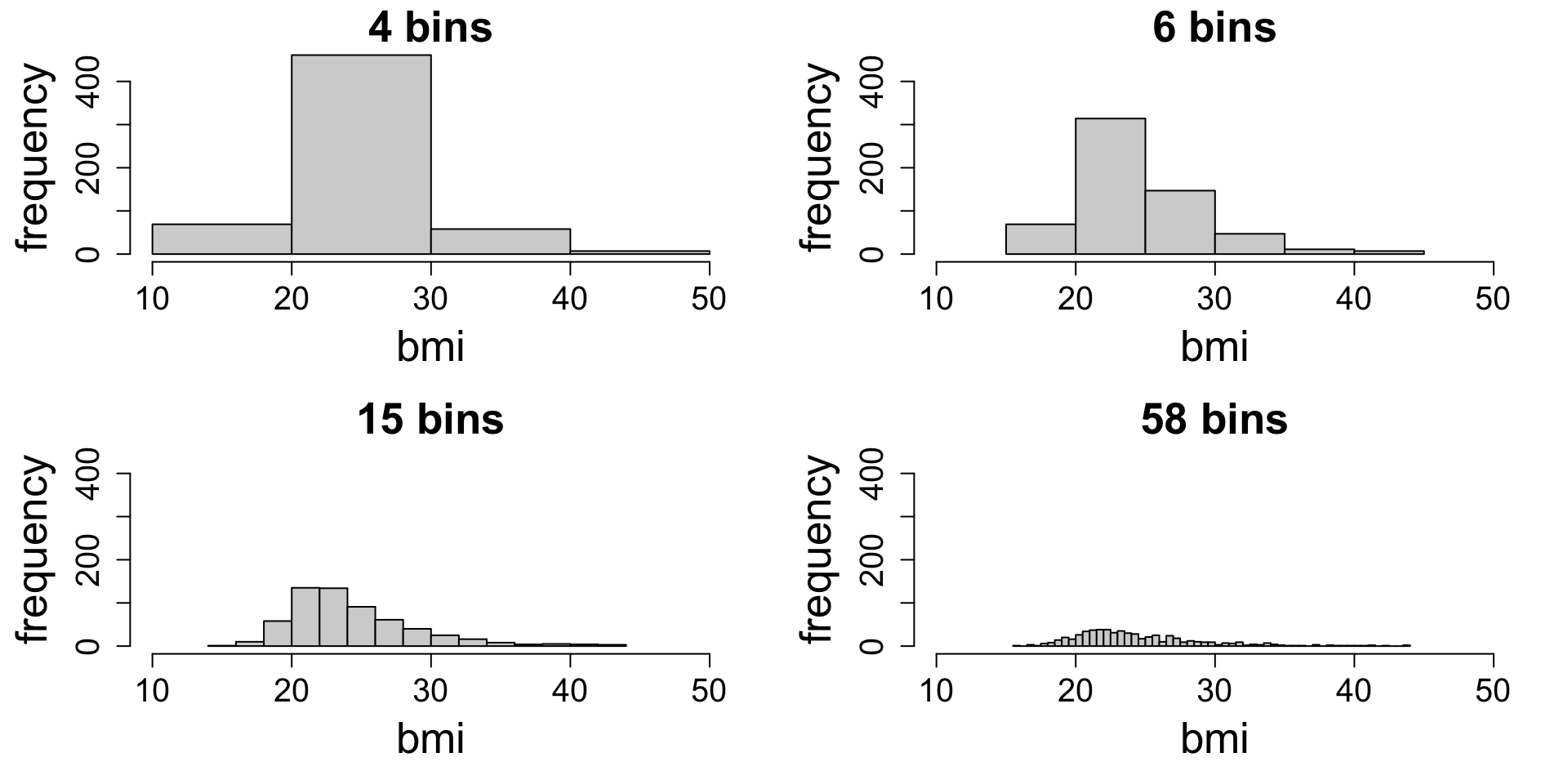
Histograms and binning
Binning has a big effect on the visual impression. Which one captures the shape best?
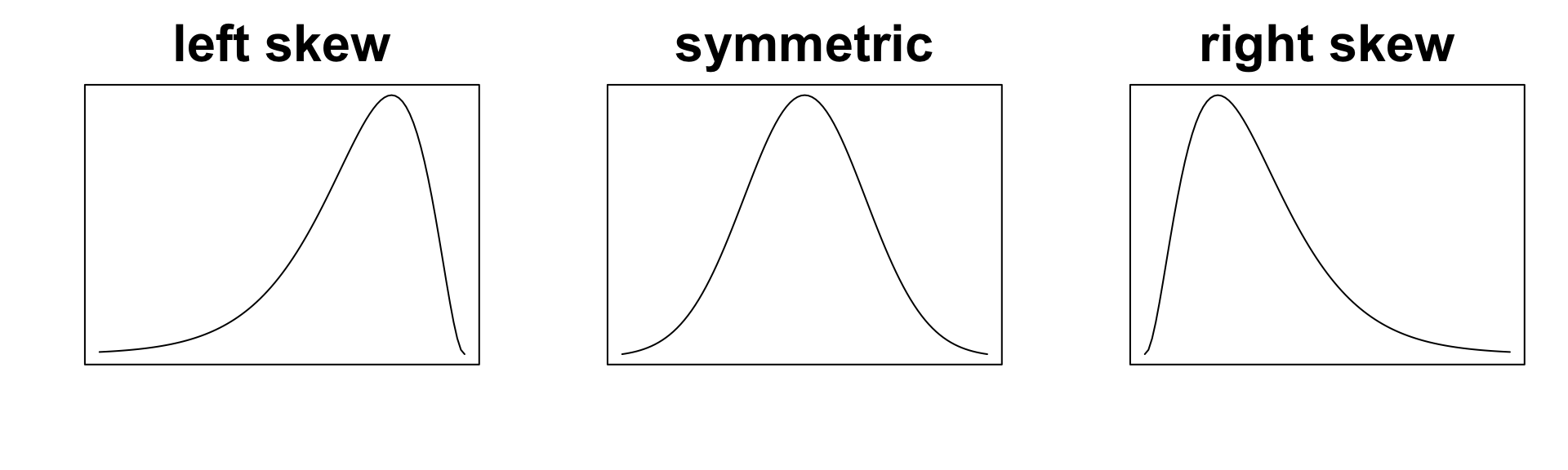
Shapes
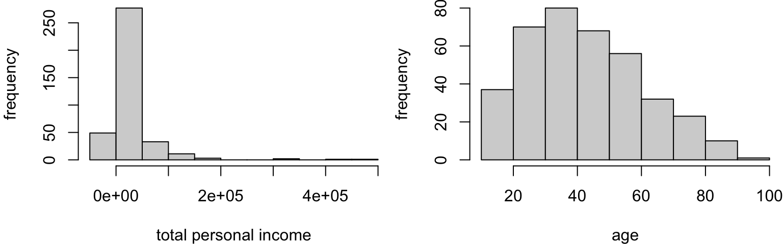
For numeric variables, the histogram reveals the shape of the distribution:
symmetric if it shows left-right symmetry about a central value
skewed if it stretches farther in one direction from a central value
Modes
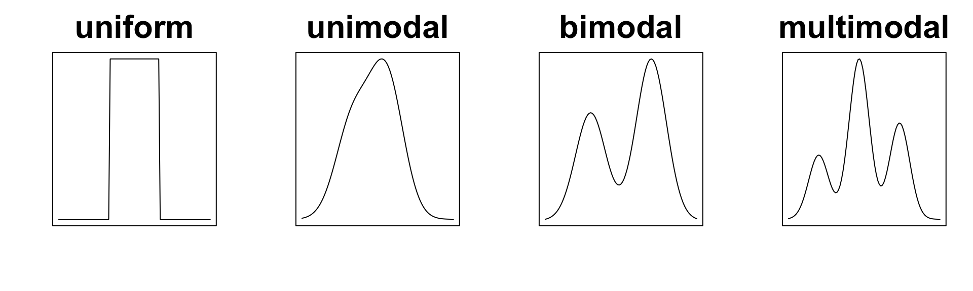
Histograms also reveal the number of modes or local peaks of frequency distributions.
uniform if there are zero peaks
unimodal if there is one peak
bimodal if there are two peaks
multimodal if there are two or more peaks
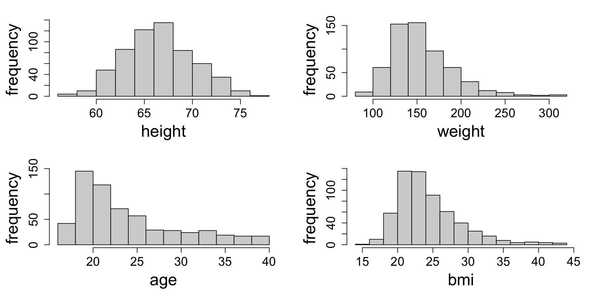
Your turn: characterizing distributions
Consider four variables from the FAMuSS study. Describe the shape and modes.
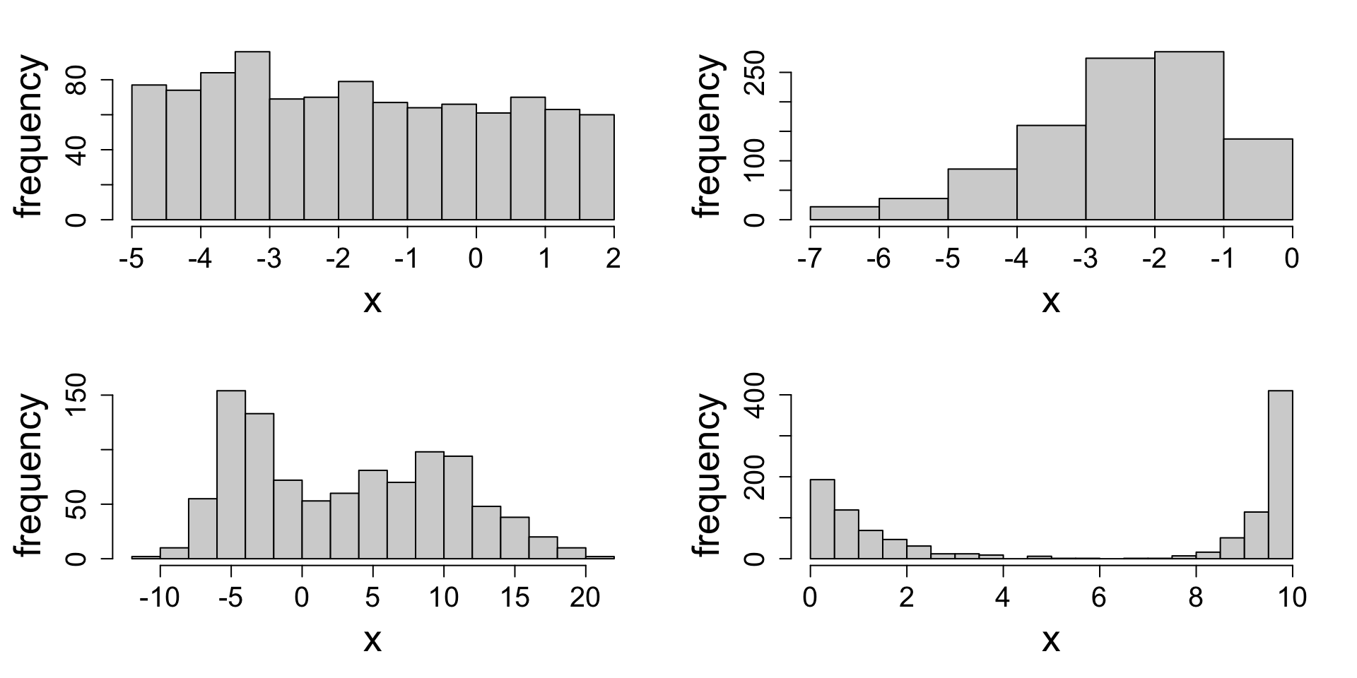
Your turn: characterizing distributions
Here are some made-up data. Describe the shape and modes.
Common statistics as measures
Most common statistics measure a particular feature of the frequency distribution, typically either location/center or spread/variability.
Measures of center:
mean
median
mode
Measures of location:
percentiles/quantiles
Measures of spread:
range (min and max)
interquartile range
variance
standard deviation
The most appropriate choice of statistic(s) depends on the shape of the frequency distribution.
Measures of center
There are three common measures of center, each of which corresponds to a slightly different meaning of “typical”:
Measure
Definition
Mode
Most frequent value
Mean
Average value
Median
Middle value
Suppose your data consisted of the following observations of age in years:
19, 19, 21, 25 and 31
the mode or most frequent value is 19
the median or middle value is 21
the mean or average value is \(\frac{19 + 19 + 21 + 25 + 31}{5}\) = 23
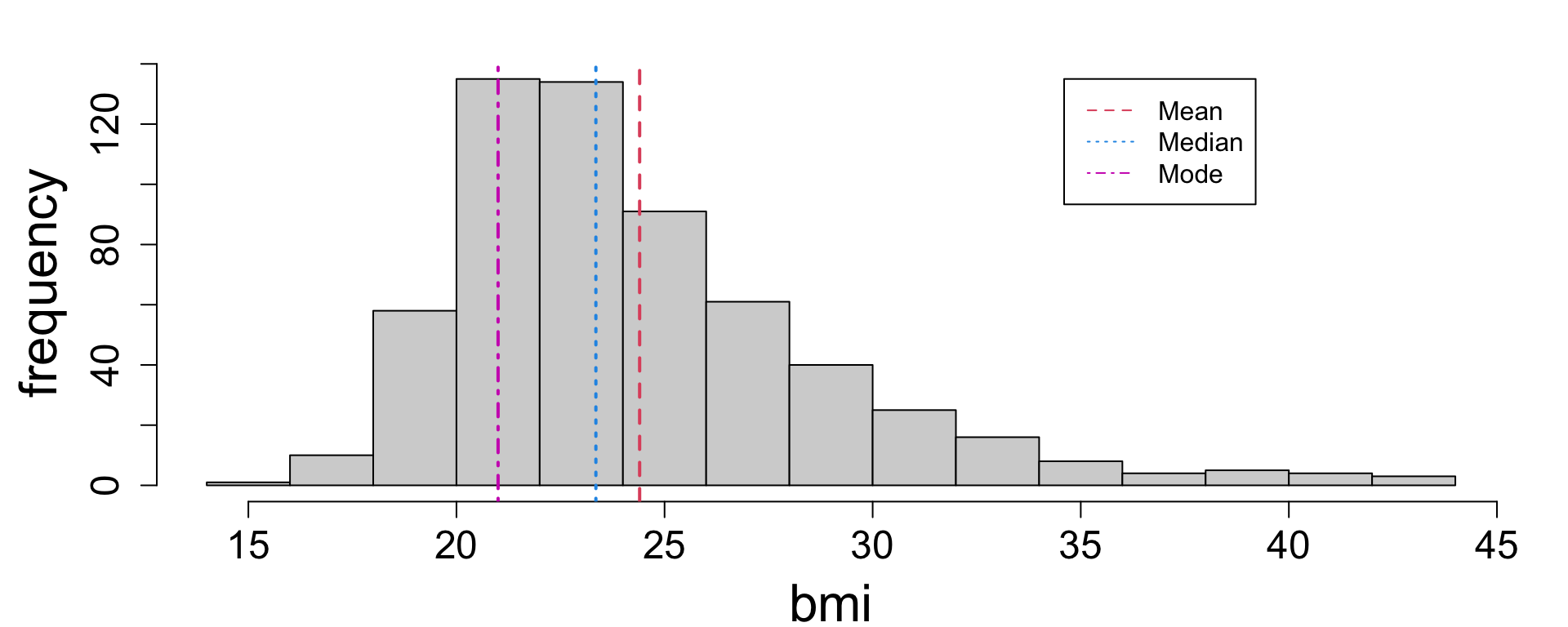
Comparing measures of center
Each statistic is a little different, but often they roughly agree; for example, all are between 20 and 25, which seems to capture the typical BMI well enough.
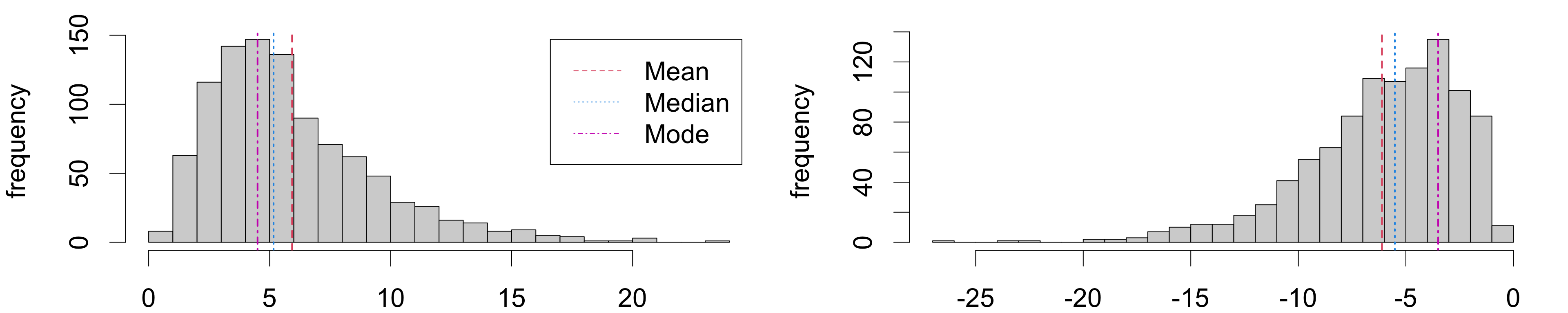
The less symmetric the distribution, the less these measures agree.
Robustness to skew
The mean is more sensitive than the median to skewness:
Comparing means and medians captures information about skewness present since:
right skew: mean \(>\) median
left skew: mean \(<\) median
symmetry: mean \(\approx\) median
For skewed distributions, the median is a more robust measure of center.
Percentiles
A percentile is a threshold value that divides the observations into specific percentages.
Percentiles are defined by the percentage of data below the threshold, for example:
20th percentile: value exceeding exactly 20% of observations
60th percentile: value exceeding exactly 60% of observations
Sample percentiles are not unique!
age
19
20
21
25
31
rank
1
2
3
4
5
Any number between 19 and 20 is a 20th percentile since it would satisfy:
20% below (19)
80% above (20, 21, 25, 31)
Usually, pick the midpoint: 19.5.
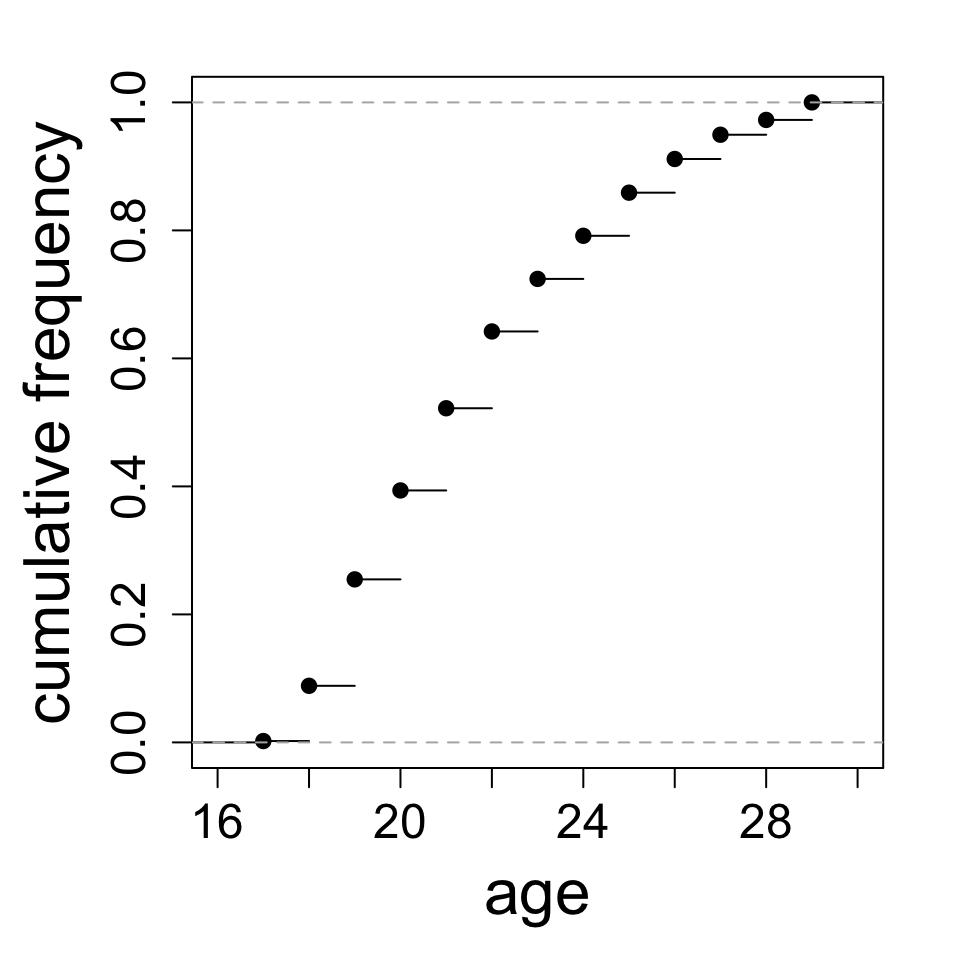
Cumulative frequency distribution
The cumulative frequency distribution is a data summary showing percentiles. Think of it as percentile (y) against value (x).
Interpretation of some specific values:
about 40% of the subjects are 20 or younger
about 80% of the subjects are 24 or younger
Your turn:
Roughly what percentage of subjects are 22 or younger?
About what age is the 10th percentile?
Common percentiles
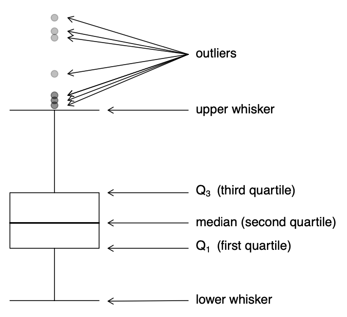
The five-number summary is a collection of five percentiles that succinctly describe the frequency distribution:
Statistic name
Meaning
minimum
0th percentile
first quartile
25th percentile
median
50th percentile
third quartile
75th percentile
maximum
100th percentile
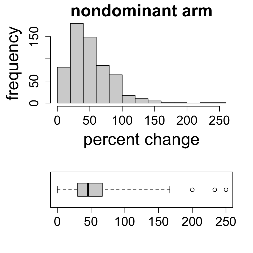
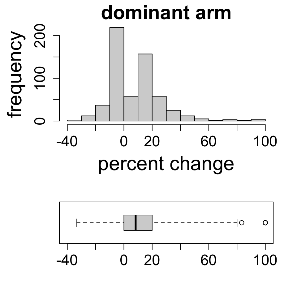
Boxplots provide a graphical display of the five-number summary.
Boxplots vs. histograms
Notice how the two displays align, and also how they differ. The histogram shows shape in greater detail, but the boxplot is much more compact.
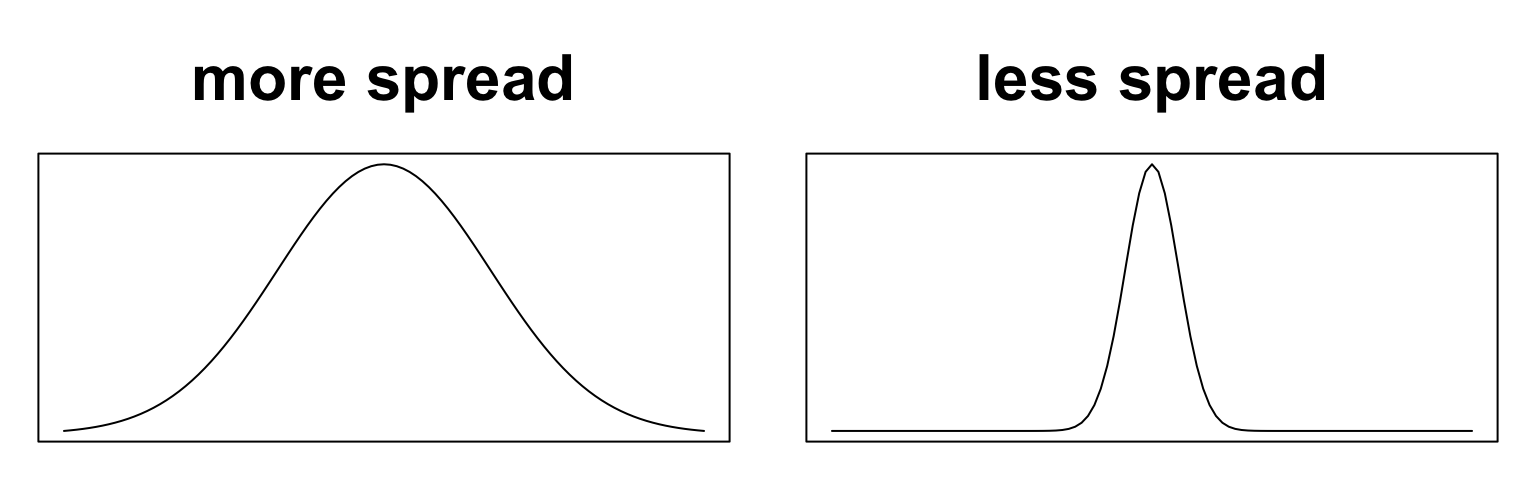
Measures of spread
The spread of observations refers to how concentrated or diffuse the values are.
Two ways to understand and measure spread:
ranges of values capturing much of the distribution
deviations of values from a central value
Range-based measures of spread
A simple way to understand and measure spread is based on ranges. Consider more ages, sorted and ranked:
age
16
18
19
20
21
22
25
26
28
29
30
34
rank
1
2
3
4
5
6
7
8
9
10
11
12
The range is the minimum and maximum values: \[\text{range} = (\text{min}, \text{max}) = (16, 34)\]
The interquartile range (IQR) is the difference [75th percentile] - [25th percentile] \[\text{IQR} = 29 - 19 = 10\]
Deviation-based measures of spread
Another way is based on deviations from a central value. Continuing the example, the mean age is is 24. The deviations of each observation from the mean are:
age
16
18
19
20
21
22
25
26
28
29
30
34
deviation
-8
-6
-5
-4
-3
-2
1
2
4
5
6
10
The variance is the average squared deviation from the mean (but divided by one less than the sample size): \[\frac{(-8)^2 + (-6)^2 + (-5)^2 + (-4)^2 + (-3)^2 + (-2)^2 + (1)^2 + (2)^2 + (4)^2 + (5)^2 + (6)^2 + (10)^2}{12 - 1}\]
Another way is based on deviations from a central value. Continuing the example, the mean age is is 24. The deviations of each observation from the mean are:
age
16
18
19
20
21
22
25
26
28
29
30
34
deviation
-8
-6
-5
-4
-3
-2
1
2
4
5
6
10
The standard deviation is the square root of the variance: \[\sqrt{\frac{(-8)^2 + (-6)^2 + (-5)^2 + (-4)^2 + (-3)^2 + (-2)^2 + (1)^2 + (2)^2 + (4)^2 + (5)^2 + (6)^2 + (10)^2}{12 - 1}}\]
In the presence of outliers, IQR is a more robust measure of spread.
Choosing appropriate measures
To determine which measures of spread and center to use, simply visualize the distribution and check for skewness and outliers.
strong skew or large outliers: prefer median/IQR to mean/SD
when in doubt, compute and compare
For example, which summary statistics are best to use below?
Inference foundations: point estimation and sampling variability
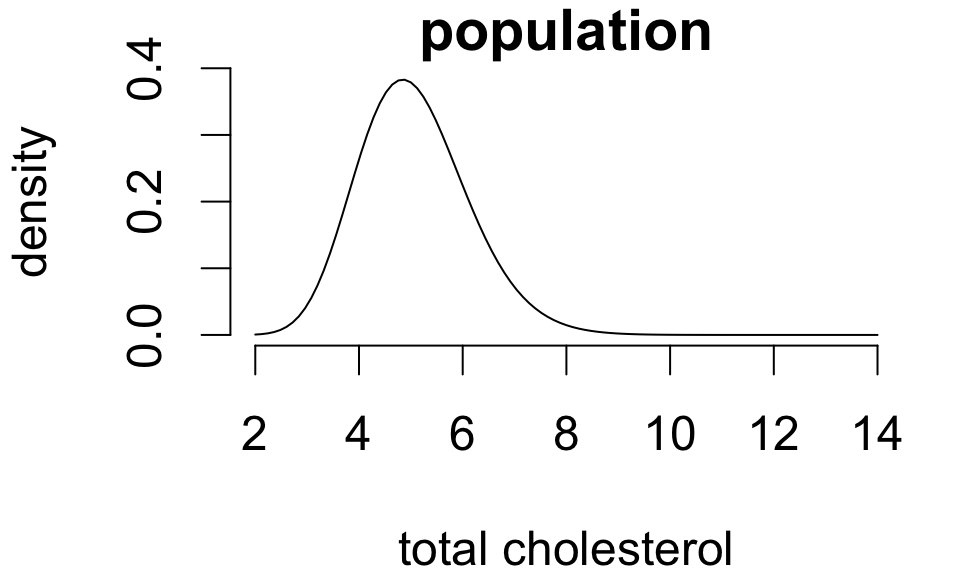
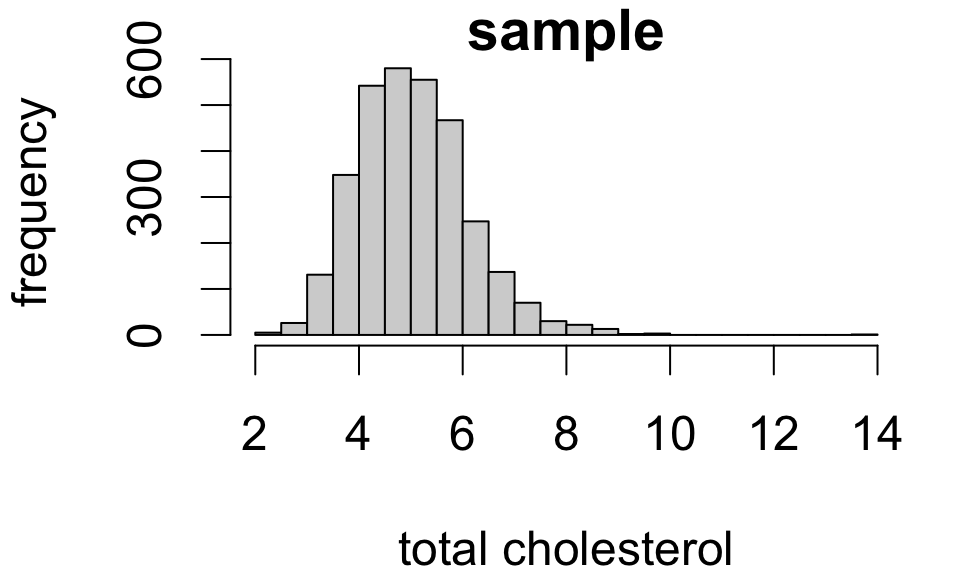
Population distributions
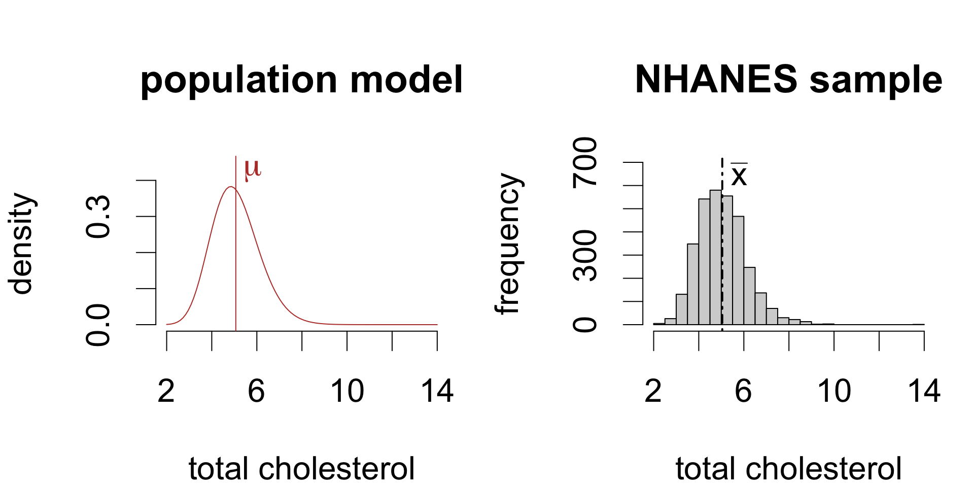
A population distribution is a frequency distribution across all possible study units.
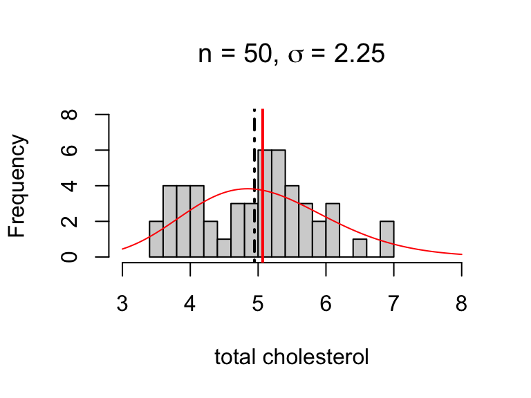
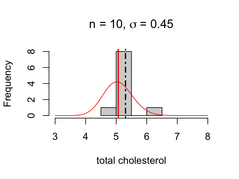
For simple random samples, the observed distribution of sample values resembles the population distribution:
The larger the sample, the closer the resemblance.1
Foundations for inference
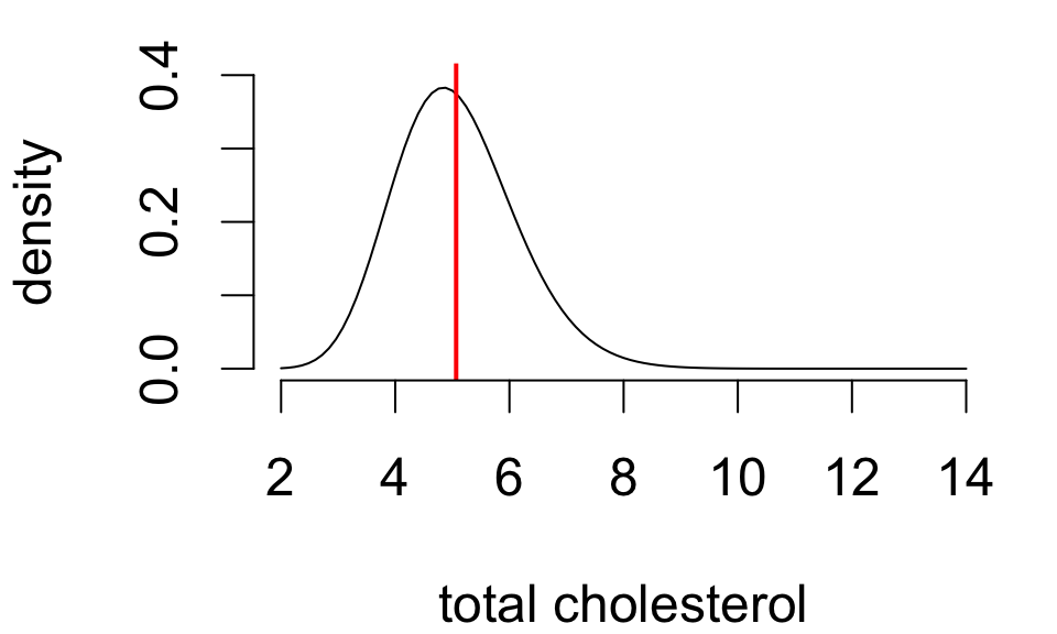
Population statistics are called parameters. These are fixed but unknown values.
Population mean
Population SD
5.067
1.126
Notation:
population mean \(\mu\)
population standard deviation \(\sigma\)
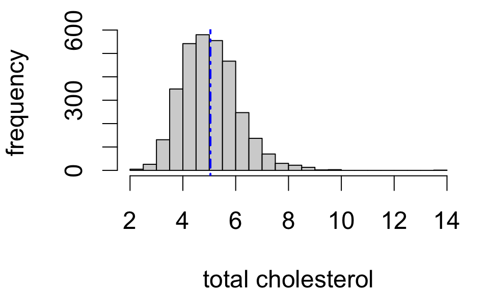
Foundations for inference
Sample statistics provide point estimates of the corresponding population statistics.
Notation:
sample mean \(\bar{x}\)
sample standard deviation \(s_x\)
Sample mean
Sample SD
Sample size
5.043
1.075
3179
Foundations for inference
Population mean
Population SD
5.067
1.126
Sample mean
Sample SD
Sample size
5.043
1.075
3179
So we might say: “mean total cholesterol in the study population is estimated to be 5.043”
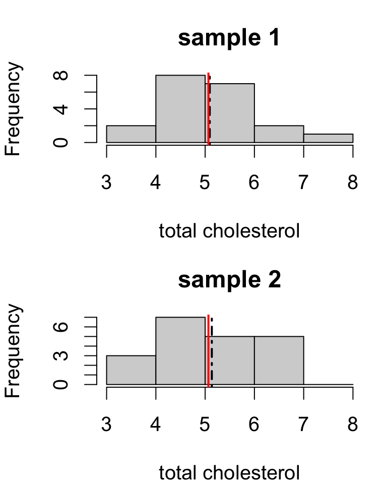
A difficulty
Different samples yield different estimates.
Sample means:
sample.1
sample.2
5.093
5.136
estimates are close but not identical
the population mean can’t be both 5.093 and 5.136
probably neither estimate is exactly correct
but both estimates should have similar errors if the study design is identical between the two samples
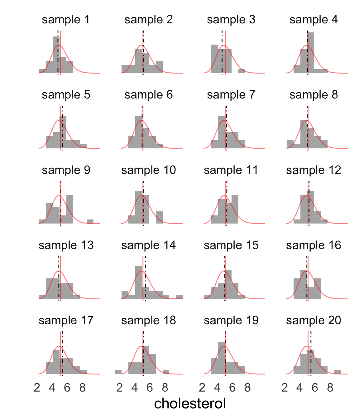
Simulating sampling variability
These are 20 random samples with the sample mean indicated by the dashed line and the population distribution and mean overlaid in red.
sample size \(n = 20\)
frequency distributions differ a lot
sample means differ some
We can actually measure this variability!
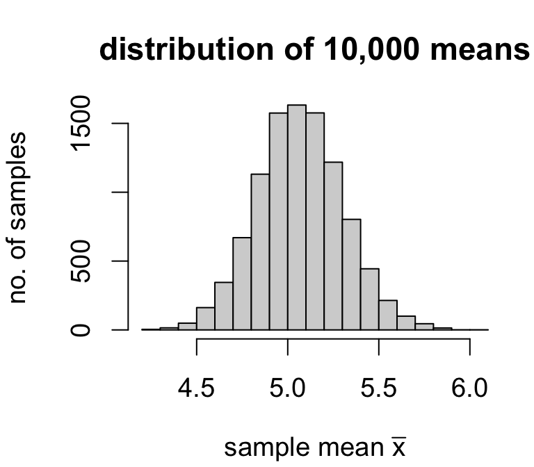
Simulating sampling variability
If we had means calculated from a much larger number of samples, we could make a frequency distribution for the values of the sample mean.
sample
1
2
\(\cdots\)
10,000
mean
4.957
5.039
\(\cdots\)
5.24
We could then use the usual measures of center and spread to characterize the distribution of sample means.
mean of \(\bar{x}\): 5.068425
standard deviation of \(\bar{x}\): 0.2369404
Across 10,000 random samples of size 20, the average estimate was 5.07 and the variability of estimates was 0.237.
Sampling distributions
What we are simulating is known as a sampling distribution: the frequency of values of a statistic across all possible random samples.
When data are from a random sample, statistical theory provides that the sample mean \(\bar{x}\) has a sampling distribution with
mean \(\color{red}{\mu}\) (population mean)
standard deviation \(\color{red}{\frac{\sigma}{\sqrt{n}}} \; \left(\frac{\text{population SD}}{\sqrt{\text{sample size}}}\right)\)
regardless of the population distribution.
In other words, across all random samples of a fixed size…
[accuracy] on average, the sample mean equals the population mean
[precision] on average, the estimation error is \(\frac{\sigma}{\sqrt{n}}\)
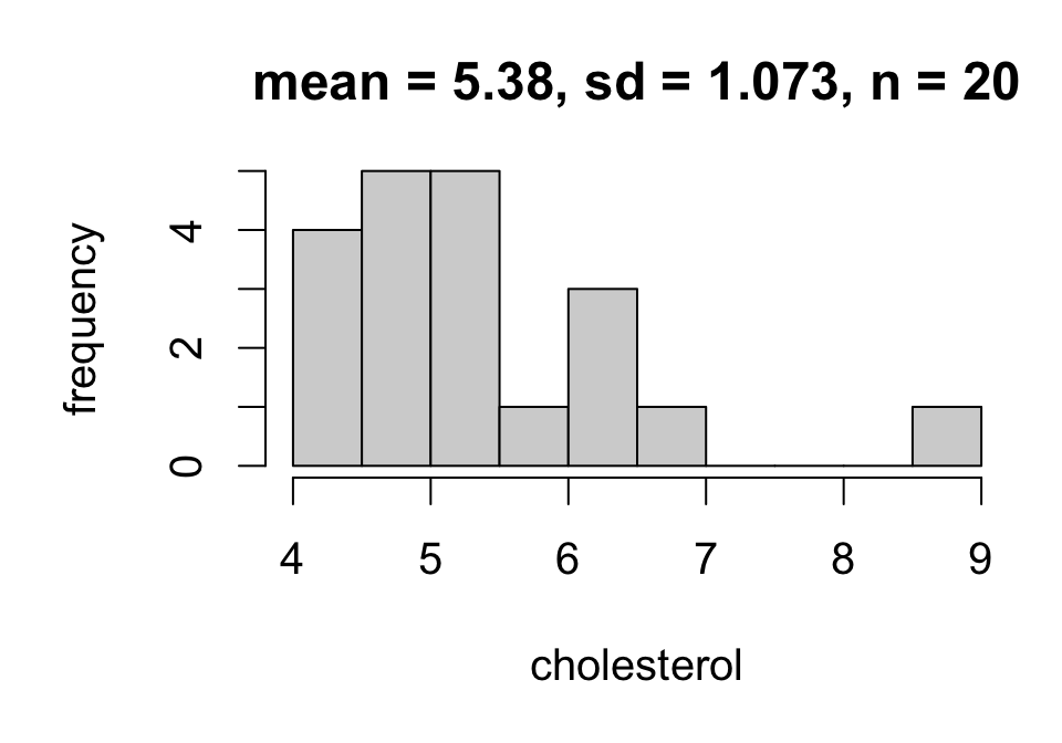
Measuring sampling variability
In practice we use an estimate of sampling variability known as a standard error: \[SE(\bar{x}) = \frac{s_x}{\sqrt{n}} \qquad \left(\frac{\text{sample SD}}{\sqrt{\text{sample size}}}\right)\]
For example:
\[SE(\bar{x}) = \frac{1.073}{\sqrt{20}} = 0.240\]
Sources of variability
There are two potential sources of variability in estimates:
population variability (\(\sigma\))
sampling variability (determined by \(n\))
For example, the estimates below are equally precise:
\(SE(\bar{x})\) = 0.1265079
\(SE(\bar{x})\) = 0.1223712
Recap
Under simple random sampling:
the sample mean \(\bar{x}\) provides a good point estimate of the population mean \(\mu\)
its estimated sampling variability is given by the standard error \(SE(\bar{x}) = \frac{s_x}{\sqrt{n}} = \frac{\text{sample SD}}{\sqrt{\text{sample size}}}\)
mean
sd
n
se
5.043
1.075
3179
0.01906
Conventional style for reporting a point estimate:
The mean total HDL cholesterol among the U.S. adult population is estimated to be 5.043 mmol/L (SE 0.0191).
Inference foundations: interval estimation
Interval estimation
An interval estimate is a range of plausible values for a population parameter.
A common interval for the population mean is: \[
\bar{x} \pm \underbrace{2\times SE(\bar{x})}_\text{margin of error}
\qquad\text{where}\quad
SE(\bar{x}) = \left(\frac{s_x}{\sqrt{n}}\right)
\]
By hand: \[5.043 \pm 2\times 0.0191 = (5.005, 5.081)\]
So the mean total cholesterol among U.S. adults is estimated to be between 5.005 and 5.081 mmol/L. Two questions:
In what sense are these values “plausible”?
Where did the number 2 come from?
The \(t\) model
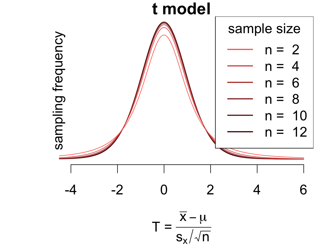
Consider the statistic:
\[
T = \frac{\bar{x} - \mu}{s_x/\sqrt{n}}
\qquad\left(\frac{\text{estimation error}}{\text{standard error}}\right)
\]
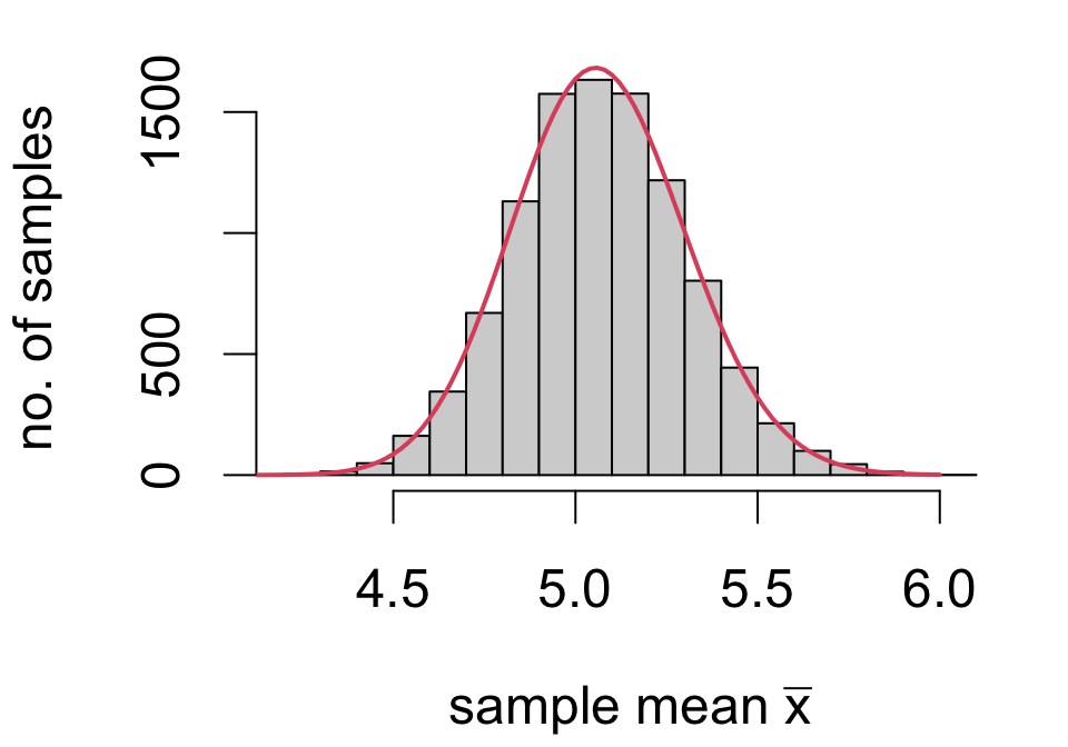
The sampling distribution of \(T\) is well-approximated by a \(t_{n - 1}\) model whenever either:
the population distribution is symmetric and unimodal OR
the sample size is not too small
Compare this with the simulated sampling distribution of \(\bar{x}\) from before – should seem plausible, since \(T\) is just \(\bar{x}\) shifted (by \(\mu\)) and scaled (by \(SE(\bar{x})\)).
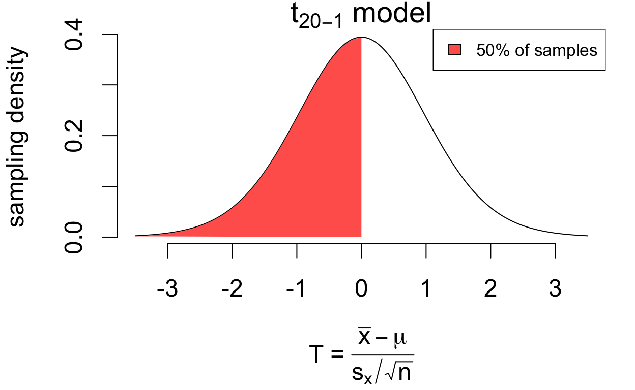
\(t\) model interpretation
The area under the density curve between any two values \((a, b)\) gives the proportion of random samples for which \(a < T < b\).
\[(\text{proportion of area between } a, b) = (\text{proportion of samples where } a < T < b)\]
For example:
for 50% of samples, \(T < 0\)
# area less than 0pt(0, df =20-1)
[1] 0.5
written as \(P(T < 0) = 0.5\)
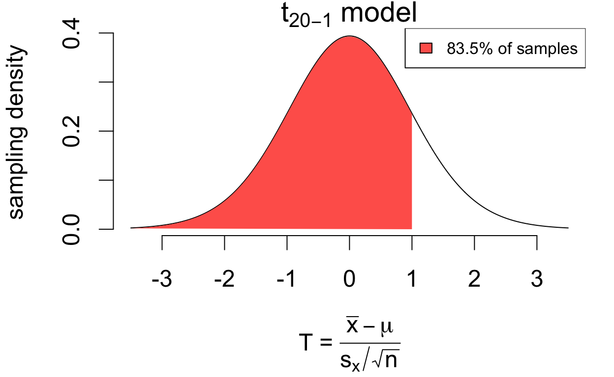
\(t\) model interpretation
The area under the density curve between any two values \((a, b)\) gives the proportion of random samples for which \(a < T < b\).
\[(\text{proportion of area between } a, b) = (\text{proportion of samples where } a < T < b)\]
For example:
for 83.5% of samples, \(T < 1\)
# area less than 1pt(1, df =20-1)
[1] 0.8350616
written as \(P(T < 1) = 0.835\)
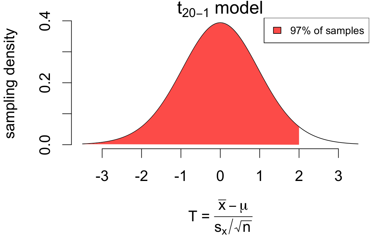
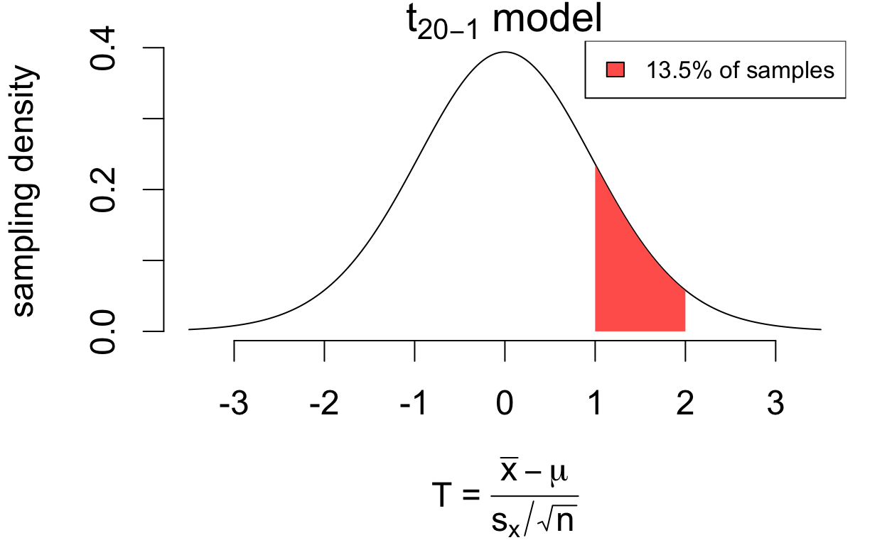
\(t\) model interpretation
The area under the density curve between any two values \((a, b)\) gives the proportion of random samples for which \(a < T < b\).
\[(\text{proportion of area between } a, b) = (\text{proportion of samples where } a < T < b)\]
For example:
for 97% of samples, \(T < 2\)
# area less than 2pt(2, df =20-1)
[1] 0.969999
written as \(P(T < 2) = 0.97\)
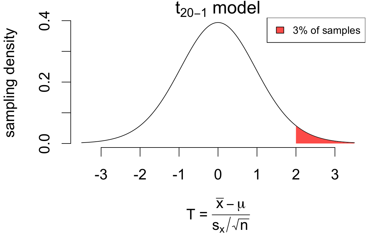
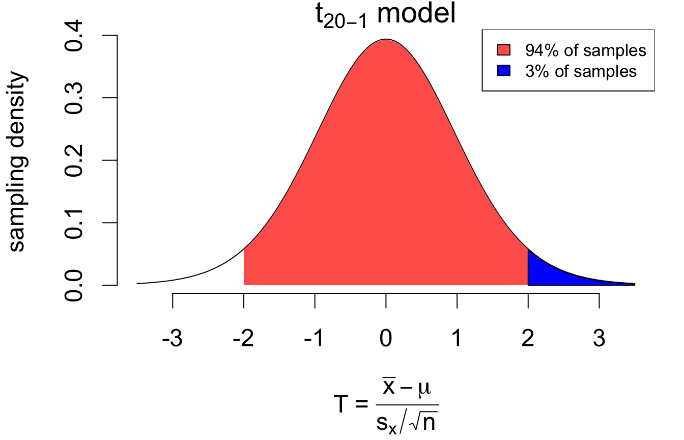
\(t\) model interpretation
The area under the density curve between any two values \((a, b)\) gives the proportion of random samples for which \(a < T < b\).
\[(\text{proportion of area between } a, b) = (\text{proportion of samples where } a < T < b)\]
For example:
for 3% of samples, \(T > 2\)
# area greater than 2pt(2, df =20-1, lower.tail = F)
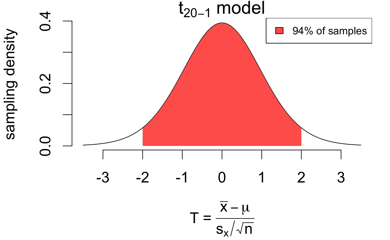
The \(\pm\) 2SE interval covers the population mean for 94% of all random samples.
So the number 2 determines the proportion of samples for which the interval covers the mean, known as its coverage.
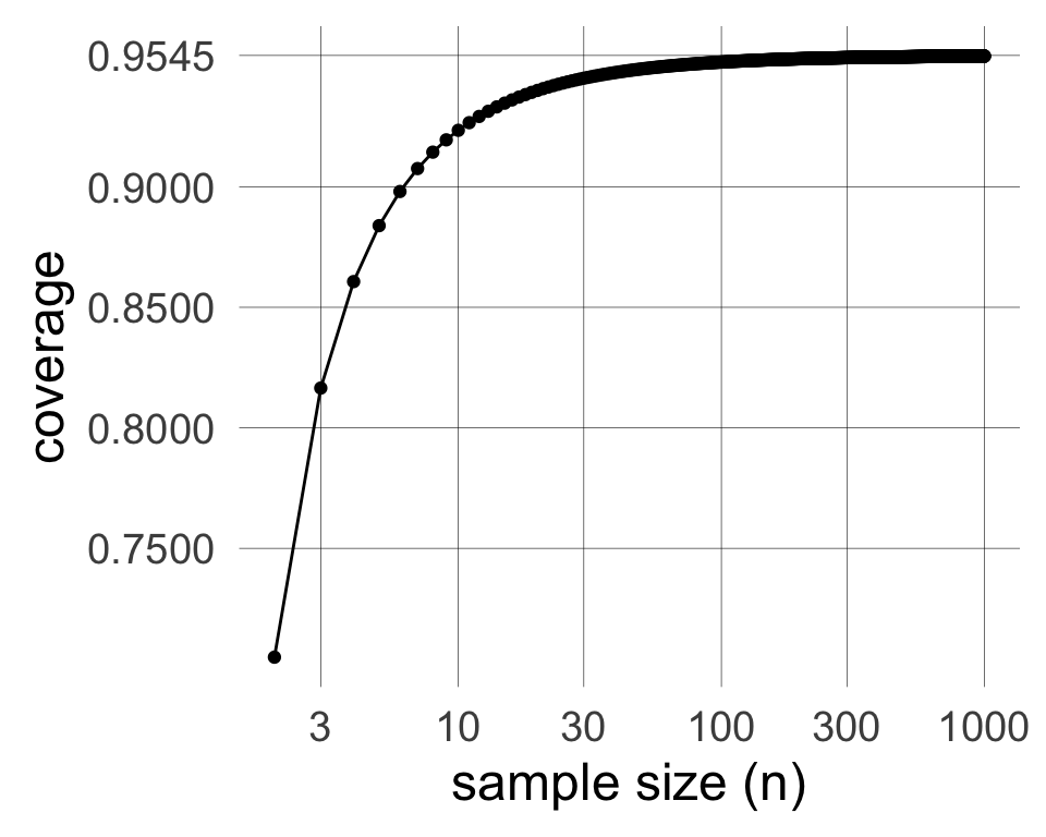
Coverage for the \(\pm\) 2SE interval
The sample size determines the exact shape of the \(t\) model through its ‘degrees of freedom’ \(n - 1\). The coverage of an interval with \(c = 2\) quickly converges to just over 95% as the sample size increases.
n
coverage
4
0.8607
8
0.9144
16
0.9361
32
0.9457
64
0.9502
128
0.9524
256
0.9534
So we use 2 standard errors by default because that gives approximately 95% coverage.
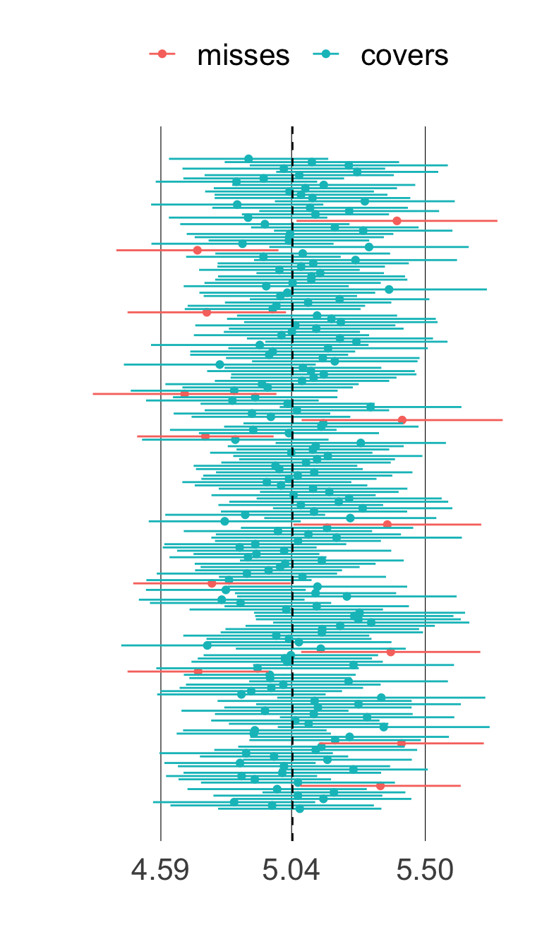
Coverage simulations
Artificially simulating a large number of intervals provides an empirical approximation of coverage.
at right, 200 intervals
94% cover the population mean (vertical dashed line)
pretty close to nominal coverage level 95%
This is also a handy way to remember the proper interpretation:
If I made a lot of intervals from independent samples, 95% of them would ‘get it right’.
Changing the coverage
Consider a slightly more general expression for an interval for the mean:
\[
\bar{x} \pm c\times SE(\bar{x})
\]
The number \(c\) is called a critical value. It determines the coverage.
larger \(c\)\(\longrightarrow\) higher coverage
smaller \(c\)\(\longrightarrow\) lower coverage
The so-called “empirical rule” is that:
\(c = 1 \longrightarrow\) approximately 68% coverage
\(c = 2 \longrightarrow\) approximately 95% coverage
\(c = 3 \longrightarrow\) approximately 99.7% coverage
Look at how the areas add up so that: \[
\begin{align}
P(\color{blue}{T > 2}) &= 0.03 \\
P(T < 2) &= 1 - 0.03 = 0.97
\end{align}
\] The critical value 2 is actually the 97th percentile (or 0.97 “quantile”) of the sampling distribution of \(T\).
So we can engineer intervals to achieve a specific coverage by going from coverage to quantile to critical value to interval.
Adjusting coverage using \(t\) quantiles
To engineer an interval with a specific coverage, use the \(q\)th quantile of the \(t_{n - 1}\) model
Note, however, that interval width depends also on the “precision” of the estimate (via \(SE(\bar{x})\)) as well as the desired coverage level.
Confidence intervals
The coverage – how often the interval captures the parameter – is interpreted and reported as a “confidence level”; we thus call interval estimates “confidence intervals”.
# ingredientscholesterol.mean <-mean(cholesterol)cholesterol.se <-sd(cholesterol)/sqrt(length(cholesterol))# 95% coverage using t quantilecrit.val <-qt(1- (1-0.95)/2, df =length(cholesterol) -1)cholesterol.mean +c(-1, 1)*crit.val*cholesterol.se
[1] 5.005566 5.080310
Conventional style for reporting a confidence interval:
With 95% confidence, the mean total cholesterol among U.S. adults is estimated to be between 5.0056 and 5.0803 mmol/L.
Recap
The “common” interval estimate for the mean is an approximate 95% confidence interval:
\[
\bar{x} \pm 2 \times SE(\bar{x})
\]
captures the population mean \(\mu\) for roughly 95% of random samples
replacing 2 with a \(t_{n - 1}\) quantile allows the analyst to adjust coverage
the \(t_{n - 1}\) model is an approximation for the sampling distribution of \(\frac{\bar{x} - \mu}{SE(\bar{x})}\)
Conventional style of report:
With [XX]% confidence, the [population parameter] is estimated to be between [lower bound] and [upper bound] [units].